"THE EFFECTS OF PAYROLL AND VALUE
ADDED TAXES ON EMPLOYMENT WITH
AN APPLICATION TO SPAIN
Richard Rogersop
Documento 87-04
Marzo 1987
A common feature of the tax systems in many OECD countries is a reliance on payroll taxes to raise revenues for government expenditure. Spain is one such country. During the period 1970-1980 there was a substantial increase in the rate at which payroll was taxed and a large number of bankruptcies and loss of employment. It is natural to question to what extent the increase in taxes was partly responsible for the concomitant decrease in employment. This paper attempts to answer that question by comparing two tax systems: one a tax on payroll, the other a tax on value added. The paper addresses the question of how much employment is affected under the two systems given that a certain amount of revenue must be raised. One novel feature of the analysis is that the model studied treats each firm as operating with a fixed coefficients technology with exogenous capacity constraints. Hence, each firm makes the decision of operating or not operating. It is shown that in the absence of heterogeneity the two tax systems are equivalent. If there is more than one type of firm then it is shown that under a reasonable condition on the correlation between productivity and profitability that a value added tax will always result in a smaller reduction in employment. Some simulations are performed which attempt to illustrate the potential magnitude of the difference in employment effects for the two tax systems. The simulations suggest that roughly twice as many jobs may have been lost because of the use of payroll tax instead of a more broadly based tax.
The economy that we study consists of a large number of firms N, each operating with a fixed coefficients technology and fixed levels of capital. There is heterogeneity across firms; each firm may have a different capital-labor ratio, different levels of capital, and different amounts of non-labor costs. A typical firm has access to the technology:
y = a in (k, a 1)
where y is output, k is a firm specific fixed level of capital, l is the amount of labor hired, and a is a firm specific parameter of the technology. The parameter a will determine the capital-labor ratio of the firm. A high value of a implies that labor is more productive and results in a higher capital-labor ratio. The intended interpretation of a is that different types of capital exist, and these different types of capital imply that production requires differing amounts of labor. It is not intended to imply that different firms have access to workers of varying skill levels, although in some cases this may be a factor of interest. Each firm faces a cost c, of operating and maintaining a unit of capital. The price of output is normalized to one and it is assumed that each firm faces a wage rate w at which it can hire labor.
Because capital is fixed, the above technology implies that firms have linear technologies with capacity constraints, i.e.
\[y = \left\{ \begin{array}{l l} a & 1, 1 \leq k / a \\ k, 1 \geq k / a \end{array} \right.\]
It follows that any firm which chooses to produce a positive amount of output will choose to produce at capacity. Hence, firms only need to make the discrete decision of operating at capacity or not operating. Each firm is defined by the parameters ( , ). If this firm operates at capacity then profits will be given by
\[\pi = k _ {1} - \omega \left[ \begin{array}{l} k _ {1} \\ - \\ a _ {1} \end{array} \right] - c k,\]
If the firm chooses to not operate then profits will be zero, Hence, the optimal decision of the firm is to operate at capacity if
(2,1)
\[\begin{array}{l} \frac {u}{\cdots + c s i} \\ a _ {i} \end{array}\]
and to not operate at all if
(2.2)
Note that for a given value of w increases in a make operation less likely, whereas decreases in a make operation less likely. This is as expected since higher values of a are associated with lower levels of productivity. Also, holding a and c constant, increases in w make operation less likely. One of the implications of this result is that holding other things constant, labor intensive firms are the first ones to drop out of the market. The above two inequalities show that the capacity of a firm is irrelevant to the decision of whether or not to operate.
For simplicity we will assume that there are n types of firms. Let be the fraction of firms which are of type i.
The purpose of this paper is to analyze different methods of raising revenue in an economy with production organized as above, and more specifically to determine the impact of different tax systems on employment. Two types of tax systems will be studied here. The first is a system where revenues are derived by taxing employer's use of labor. This corresponds to the Social Security Tax which is currently used in Spain to generate a large amount of total tax revenue. The second tax system considered is one in which the tax is levied on the value added of each firm. In the model described above value added is simply the output of a firm.
For future reference it is of interest to derive the connection between the a, parameters and labor's share of value added. If a firm is operating at capacity then total value added is given by k, and payments to labor are given by
w k/a. Hence labor's share of value added is given by
Hence, in condition (2.1) and (2.2) the first term is simply labor's share of value added. Empirically it turns out that it is enough to know the value of this parameter without explicitly knowing the value of . Note that a necessary condition (although clearly not sufficient) for operation at capacity to be optimal is that w/a, be less than one. Note that is the marginal product of labor for production less than or equal to capacity, so that this condition is simply saying that the wage must be less than or equal to the marginal product of labor in order for production to take place.
3. ANALYSIS OF DIFFERENT TAX SYSTEMS
We begin the analysis by solving for the equivalent conditions for (2,1) and (2,2) in the case where taxes are present. Consider first the case of a tax on labor, denoted by . If a firm defined by the parameters ( , ) operates at capacity, then its profits will be given by:
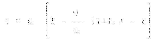
which means that the condition for operation versus closing down becomes operate if
\[(3, 1) \frac {w}{5}, (1 + 1) + c \leq 1\]
and close down if
\[(3, 7) \frac {0}{a _ {i}} - (1 + t _ {i}) + c > 1\]
Now consider the case of a tax on value added. Denoting this tax by , a firm defined by the parameters ( , ) operating at capacity will now have profits defined by:
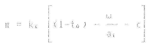
The conditions for operation now become operate if
(3,3)
\[\begin{array}{l} \frac {U}{\partial_ {1}} + C \leq 1 - t _ {0} \\ \partial_ {1} \end{array}\]
and close down if
(3, 8)
\[\begin{array}{l} \text { 0 } \\ \text { 3 , } \end{array} \quad \text { 4 } \quad \text { 5 } \quad \text { 1 } \quad \text { 2 } \quad \text { 3 },\]
Revenues and employment under the two systems are of interest and expressions for them are given by:
\[\beta_ {1} = \sum_ {i} t _ {i} \frac {\omega}{a _ {i}} k _ {i}\]
\[E _ {1} = \sum_ {i} \frac {k _ {i}}{q _ {i}}\]
where in the above expressions, the sum is over all i satisfying condition (3,1). For the value added tax we have:
\[(3, 7) \quad R _ {0} = \sum_ {i} L _ {0} K,\]
(3.8)
Where in these two expressions the sum is over all i satisfying condition (3.3)
3.1 An Economy With One type of Firm
The first case we consider is an economy in which all firms are the same. This case is of interest because it turns out that the presence of heterogeneously is crucial in understanding the difference between the two systems. In the case where all firms are identical we will show that there is no difference between the two tax systems in terms of their ability to raise revenues. To see this suppose that all firms have parameter values equal to (k, a). Assume that the wage was such that operation produces positive profits for these firms, i.e., assume
Because all firms are the same it follows that either all firms produce or no firms produce (Note that throughout the analysis we will assume that marginal firms produce, i.e., that a firm with zero profit will continue to stay in operation. This assumption is not critical to any of the results but it simplifies the exposition by not requiring the use of limiting arguments as the zero profit condition is approached). The question we address is the following: what is the maximum amount of revenue that can be obtained through each of the tax systems without forcing the firms on the economy to not operate. In the absence of any taxes profits of each firm are given by
\[\mathbf {n} = k \left[ \begin{array}{c c c} & 0 & \\ 1 & \dots & 0 \\ 1 & 0 & \end{array} \right]\]
The answer to the above question is that in each case it is possible to tax away all of the profit. It doesn't make any difference which system is used. Each system will tax the profit away in a different manner, but the final outcome will be the same. Referring to conditions (3.1) - (3.4), the maximum tax rate on labor which is consistent with the firms remaining in operation is given by
\[i _ {1} = \frac {i - c - w / a _ {1}}{w / a _ {1}}\]
From equation (3.5) this produces total revenue given by
which is simply the total profit in the economy. On the other hand, from equation (3.3) the maximum tax on output (or value added) which is consistent with the firms remaining in operation is given by
and from equation (3.7) this produces a revenue of
which again is simply the total profit in the economy.
The intuition behind this result is very simple. This is an economy in which there are no marginal decisions being made - the only decision being made is the non-marginal decision of whether or not to operate. Hence, independently of the method of taxation it is possible to tax away all profit without affecting any decisions.
This result will continue to hold even if firms have different values of k, but the same values of c and a. Hence, the result does not depend on all firms being the same size but does require that all firms have identical unit labor
costs (or capital-labor ratios) and the same cost of capital.
3.2. An Economy With Two Types of Firms
Before turning to the general case it is instructive to look at the case where there are two types of firms. The intuition in this case is identical to that in the more general case. To simplify exposition we assume that so that the only difference between the two kinds of firms is their values of a. Assume that , with this specification it is always the case that firms of type one will stop operating before firms of type two stop operating, let us begin by asking how much revenue each of the two systems can raise without causing any firms to shut down. We assume that w/a, < 1.
Requiring that no firms shut down will impose a restriction on how big tax rates can be. It will be the parameters defining type one firms that set the upper limits on tax rates since they are the first firms to close down. In the case of a tax on labor the maximum tax will be given by
1 - w/a1 - c
i.
and this will produce a revenue of
\[K _ {1} = p _ {1} N \left[ 1 - \frac {\omega}{a _ {1}} - c \right] + p _ {2} N \left[ 1 - \frac {\omega / a _ {1} - c}{a _ {2} / a _ {1}} \right]\]
In the case of a tax on output the maximum tax rate is
\[t _ {0} = 1 - w / a _ {1} - c\]
which will produce revenues of
\[S _ {0} = p _ {1} N \left[ 1 - \frac {U}{a _ {2}} - c \right] + p _ {2} N (1 - u / a _ {3} - c)\]
Comparing the expressions for and it can be seen that the first term in each expression is the same. However, the second terms differ because the second term in the expression for contains the term in the denominator. By assumption , so this term is greater than one. It follows that less revenues will be raised by the tax on labor. To gain some additional insight into what is causing this result to occur, look at the
amount of revenue that is being raised per firm according to type in each of the two tax regimes. In the labor tax case, each firm of type one pays (i - w/a; - c) whereas each firm of type two pays (i - w/a; - c)
(32/8)
In the case of an output tax each of the firms is contributing an amount equal to (1 - w/a - c). Why is if that in one case firms contribute equal amounts but that this is not true in the other case? In the case of a tax on labor the tax has a different impact on firms depending upon how much labor they use. Or more importantly, the relative impact of a tax on labor depends upon the capital to labor ratios. Hence, firms with low values of this ratio suffer relatively more than do firms with high values of this ratio. In the above example firms of type two have higher values of the capital to labor ratio, which means that firms of type two are contributing relatively less. This does not happen in the case of a tax on output. This tax does not discriminate between firms with different capital to labor ratios. Put another way, in the case of a tax on labor firms contribute differently per unit of capacity depending upon their capital to labor ratio, whereas in the case of the output tax all firms contribute the same per unit of capacity. The reason that this is important has to do with the order in which firms leave the market. Firms with higher capital-labor ratios are the last ones to leave. Hence, if we take the marginal category of firms (i.e., those with zero profit), then all firms with higher profits will have higher capital-labor ratios and will be contributing a smaller amount to tax revenues. Although both types of taxes can tax sway all profit from a given group of firms, the payroll tax is less effective at raising revenue from the non-marginal groups because it is their low shares for the value added by labor which makes them profitable.
It should be clear that the above conclusion will continue to hold even if the capacity of type one and two firms are different.
Now consider the question of how much revenue can be raised from each system assuming that taxes are raised to the point where type two firms operate but type one firms don't. In this case there is no revenue from type one firms and it is only the profitability of type two firms that matters. This reduces to the case where there is only one type of firm studied above. Note that in this type of economy it is certainly not the case that higher tax rates imply higher revenues. In general as taxes are raised some firms stop operating causing the tax base to decrease.
3.5 Firm Specific Cost of Capital
We now extend the analysis to allow for the values of c to be firm specific. The motivation for wanting to allow such a feature arises from the fact that different values of a are interpreted as selecting different types of capital or different methods of production, if this is true, then it is natural to allow the values of c to also vary. It turns out that allowing arbitrary values for the c, will cause the previous results to no longer hold. This is demonstrated via an example. Afterward a reasonable assumption is made under which the preceding results will continue to hold.
Example: Consider an economy with only two types of firms. The values of are given by:
15
Firm 1 2 1 .1 Firm 2 4 1 .4
Assume , and
First we find the maximum revenue consistent with all firms operating. In this example it turns out that firms of type one are not the first firms to drop out of operation in response to increases in the output tax, although they are the first ones to drop out in response to increases in the payroll tax. If all firms are to remain in operation the maximum value of the payroll tax is given by
i: = .8
and the maximum value of the output tax is given by
to = .35
Revenues are then given by
Since the labor tax generates more revenue for a given level of employment it follows that the converse is also true, namely that for some revenue constraint the labor tax will result in a higher level of employment.
Previously it was shown that if c is constant across firms then this result would never happen. We will now show that there is something undesirable about the nature of the example and show that once this feature is eliminated so is this result. The undesirable feature of this example is the correlation between productivity and net profit per unit of capital. Average product of labor is positively correlated with the value of a. For firms producing the same product it is natural to expect a positive correlation between profitability and productivity, given that wages are constant across firms. Profit per unit of capital is given by
For the above example it is possible to show that
31; = .
so that firms of type two have higher productivity but are less profitable. In the example this happens because is sufficiently larger than . If we impose as a restriction that the value of a and net profitability per unit of capital are positively correlated then this result will not happen. The important implication of this assumption is that for both types of taxes it will always be the case that firms with low values of a are the first to drop out of operation. We show this formally:
Claim: If and are positively correlated and then if firm is operating so is firm , for both kinds of taxes.
Proof: First consider the tax on output. Profits per unit of capital are given by
π = (1) ... (2) ... 0 ... C ... ... ... ... ... ... ... ...
By assumption (w/a + c) is negatively correlated with a. Since the first terms are identical it follows that iff .
Now consider the case of a tax on labor. Profits per unit of capital are now given by:
= 1 - ω = 3, (1 + t_{1}) = c_{1}
If a and w/a + c are negatively correlated it is still true that a and w/a (1+t) + c are negatively correlated, because the term being added is t:w/a and this is negatively correlated with a.
Note that in the example this property was violated, and it is this violation that causes the result: because type one firms have higher profit than type two firms the fact that type one firms are marginal for the payroll tax whereas type two firms are marginal for the output tax means that the payroll tax raises more revenue from the marginal group. If both taxes have the same type of firm as the marginal firm then both necessarily raise the same revenue from the marginal group, and the output tax raises more revenue from other groups. Hence the output tax is more effective at raising revenue.
In this section we prove the following preposition:
Proposition: If a and w/a + c are negatively correlated then the output tax always results in employment at least as great as the payroll tax for a given revenue constraint.
Proof: The proof follows the same logic as the case of two types of firms. We show that for any level of employment the output tax always has revenue which is at least as large, we have previously established that the firms can be ranked according to their values of a so that firms with lower values of a are the first to stop producing. Assume . First we calculate maximum revenues from the two taxes assuming all firms remain in operation, maximum tax rates consistent with this are
Revenues will then be given by:
\[R _ {i} = p _ {i} N k _ {i} \left(1 - \omega / a _ {i} - c _ {i}\right) + \sum_ {Z} (p _ {i} N) k _ {i} \frac {\omega}{a _ {i}} \left[ \begin{array}{c} 1 - c _ {1} - \omega / a _ {1} \\ \hline \omega / a _ {2} \end{array} \right]\]
\[= p _ {i} N k _ {i} \left(1 - \omega / a _ {i} - c _ {i}\right) + \sum_ {2} ^ {N} (p _ {i} N) k _ {i} \left[ \frac {1 - c _ {i} - \omega / a _ {i}}{a _ {i} / a _ {i}} \right] ^ {- 1}\]
\[= N (1 - \omega / a _ {1} - c _ {1}) \left[ \begin{array}{l l} N & a _ {2} \\ \sum p, k _ {2} & - \\ 1 & a _ {3} \end{array} \right]\]
\[K _ {0} = p _ {1} N k _ {1} \left(1 - w / a _ {1} - c _ {1}\right) + \sum_ {2} ^ {M} (p _ {1} N) k _ {1} \left[ \begin{array}{c c c} & 0 \\ 1 & - & - c _ {1} \\ 1 & a _ {1} \end{array} \right]\]
\[= N (1 - \omega / a _ {1} - c _ {1}) \left[ \begin{array}{l l l} 1 & & \\ 2 & p _ {1} & k _ {1} \\ 1 & & \end{array} \right]\]
As in the two form case, note that the first term in the summation is the same for both taxes, but for , all the terms in the output tax revenues are larger because is for .
This argument can be repeated for any level of employment. If the first i-l types of firms do not operate then maximum taxes and revenues are given by:
\[i _ {1} = \frac {i - c _ {1} - w / 3}{w / 3}\]
\[i _ {0} = i - w / a, \dots c,\]
\[N _ {1} = N (1 - \omega / a _ {1} - c _ {1}) \left\{ \begin{array}{l l} 1 & a _ {1} \\ \sum p _ {j} & k _ {j} \\ 1 & a _ {j} \end{array} \right.\]
\[\hat {K} _ {i j} = N (1 - \omega / 3, - c _ {j}) \left[ \begin{array}{l l l} \Pi & & \\ \sum_ {j} \rho_ {j} & k _ {j} \\ 2 & & \end{array} \right]\]
The same conclusion applies. This completes the proof of the proposition.
In this section we perform some simulations of the previous model, with the distribution chosen to correspond to the Spanish economy. As noted earlier in the paper the relevant information that is needed to simulate the model is the distribution of employment by firms according to labor's share of value added. We will assume that the parameter c is the same for all firms and as well set it equal to zero. Setting c equal to some other value is not going to affect the results in any significant manner because c affects the decision of operating or not operating in the same manner in both tax systems: it simply reduces profits per unit of capacity by the amount c. The parameter c essentially scales before tax profits. Since we are interested in comparing the two tax systems for a given value of c it does not matter what the level of pretax profits are. This level of pretax profits will affect the amount of revenue a particular tax system can raise but it will not affect the relative revenues raised by two different tax systems when the value of c is independent of the tax system.
In order to get an approximate distribution of labor's share of value added for the Spanish economy we used the data contained in the Central de Balances del Banco de España. We used data on firms in Construction, Glass and Ceramics, Chemicals, Metals (except transportation), Food and Manufacturing except for Food for the year 1931. This survey gives information on employment and labor's share of value added at the firm level. For the above sectors there are observations convering 1292 firms. Because the model of the previous section predicts that all firms with a given labor share of value added drop out at the same time it is enough to aggregate the data as if there were only one firm in any particular category of labor share of value added. We considered twenty groups each with a range of .05 in labor's share. Table One contains the summary information from this survey.
This information can be used as a guideline to assist in choosing parameters for the simulations. A few points of warning must be noted. First, that this data is for 1981, which is ten years after the increases in taxation started. Theory predicts that the increase in taxation over the period 1970-1980 affects the distribution of firms in operation. Second, in the model of the previous sections a firm will always have the same labor share in value added (assuming wages and prices are constant). In the actual economy individual firms in a particular year may be affected by a large number of idiosyncratic factors. If adjustments to labor are costly, firms may have highly volatile series for labor's share of value added. Hence, any particular cross-section gives at most some approximate distribution. Finally, if disequilibrium factors are important, i.e. if firms are constrained in the output market, then this will also affect the distribution.
TABLE ONE DATA FROM CENTRAL DE BALANCES DEL BANCO DE ESPAÑA FOR 1981
| Labor's Sharein Value Added | No. ofFirms | TotalEmployment | Share in TotalEmployment | Share in TotalValue Added |
| 0.00 - 0.05 | 0 | 0 | 0.0 | 0.0 |
| 0.05 - 0.10 | 2 | 162 | 0.0 | 0.0 |
| 0.10 - 0.15 | 13 | 648 | 0.1 | 0.3 |
| 0.15 - 0.20 | 20 | 4,959 | 1.0 | 2.8 |
| 0.20 - 0.25 | 25 | 3,757 | 0.7 | 1.6 |
| 0.25 - 0.30 | 33 | 7,656 | 1.5 | 2.2 |
| 0.30 - 0.35 | 48 | 10,308 | 2.1 | 3.4 |
| 0.35 - 0.40 | 72 | 27,108 | 5.4 | 7.5 |
| 0.40 - 0.45 | 103 | 36,260 | 5.2 | 6.5 |
| 0.45 - 0.50 | 133 | 51,649 | 10.2 | 11.4 |
| 0.50 - 0.55 | 173 | 80,005 | 13.3 | 14.0 |
| 0.55 - 0.60 | 175 | 73,015 | 14.4 | 13.4 |
| 0.60 - 0.65 | 167 | 79,563 | 15.7 | 13.4 |
| 0.65 - 0.70 | 171 | 74,220 | 14.8 | 11.0 |
| 0.70 - 0.75 | 67 | 30,340 | 6.0 | 4.5 |
| 0.75 - 0.80 | 41 | 14,795 | 7.9 | 2.0 |
| 0.80 - 0.85 | 32 | 8,303 | 1.7 | 1.1 |
| 0.85 - 0.90 | 19 | 5,132 | 1.0 | 0.6 |
| 0.90 - 0.95 | 7 | 1,477 | 0.3 | 0.2 |
| 0.95 - 1.00 | 7 | 5,543 | 1.0 | 0.6 |
In any event, the information in table one suggests that the distribution of total value added by category of labor's share in value added is single peaked with a peak in the range .5 - .55. It is also skewed to the right. To simplify the simulations we have used distributions which have single peaked density functions with two linear pieces. The generic form used is:
\[f (v) = \left\{ \begin{array}{l l} 0 & \text { for } v \leq v _ {1} \\ a _ {1} & (v - v _ {1}) \text { for } v _ {1} \leq v \leq v _ {2} \\ a _ {2} & (v _ {2} - v _ {1}) - a _ {3} (v - v _ {2}) \text { for } v _ {2} \leq v \leq v _ {3} \\ 0 & v \geq v _ {3} \end{array} \right.\]
This is a distribution with the following forms:
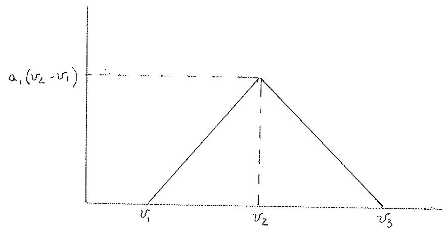
labor's share above vs, We have used three different sets of parameters:
| $V_1$ | $V_2$ | $V_3$ | $3_1$ | $3_2$ | |
| Case 1 | .20 | .60 | 1.00 | 6.25 | 6.25 |
| Case 2 | .20 | .65 | 1.00 | 5.56 | 7.14 |
| Case 3 | .20 | .70 | 1.00 | 5.00 | 8.39 |
Note that once , and are chosen there are unique values of and which make a porper density (i.e., which make integrate in one).
For each of these cases we choose tax rates to and in which result in a range of values for employment and calculate the ratio of the revenues produced by the low tax systems. These results are given in tables two-seven, in these tables the variables with the number one refer to payroll tax and the variables with the number two refer to the output tax,
Integrating the distribution for f(v) gives the following formulas:
\[\text {EMPI} = \left[ \begin{array}{l l l l l} 1 & & & & \\ 1 + t _ {1} & & & & \\ 0 & f (v) & d v & = \frac {a _ {1}}{2} & (v _ {2} - v _ {1}) ^ {2} + a _ {1} (v _ {2} - v _ {1}) \\ 0 & & & & \end{array} \right] \left[ \begin{array}{l l l} 1 & & \\ \frac {1}{1 + t _ {1}} & - & v _ {2} \\ 0 & & \end{array} \right] = \frac {a _ {2}}{2} \left[ \begin{array}{l l l} 1 & & \\ \frac {1}{1 + t _ {1}} & - & v _ {2} \\ 0 & & \end{array} \right] 2\]
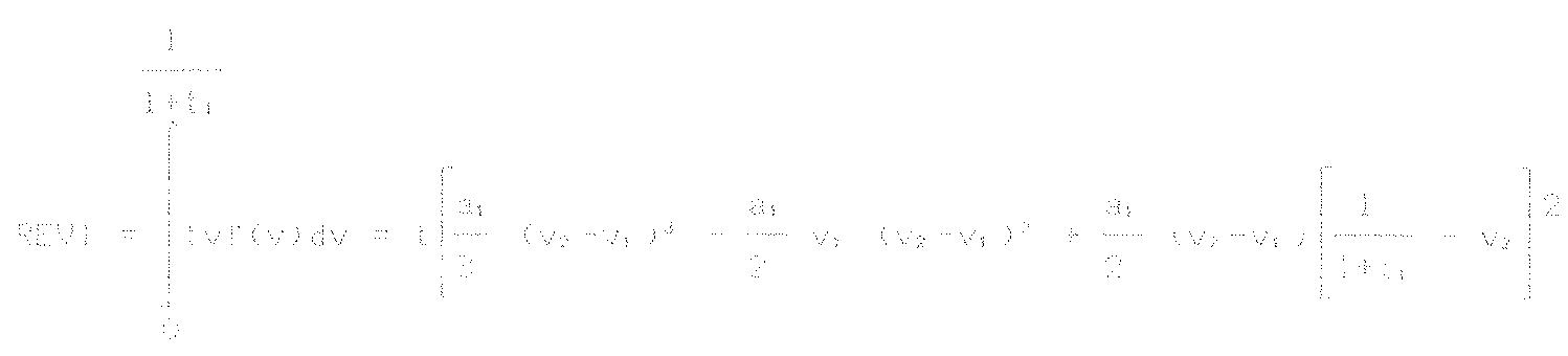
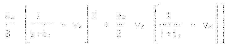
\[\text {CHP2} = \int_ {0} ^ {1 - t _ {0}} f (v) d v = \frac {a _ {1}}{2} (v _ {2} - v _ {1}) ^ {2} + a _ {1} (v _ {2} - v _ {1}) (1 - t _ {0} - v _ {2}) - \frac {a _ {2}}{2} (1 - t _ {0} - v _ {3}) ^ {2}\]
\[R E V 2 = \int_ {0} ^ {1 - t _ {0}} t (v, d v = 1) D P 2\]
CASO 3
| Ti | EMP1 | REV1 | REV2/REV1 |
| 0 | 1,000 | 0,00 | |
| 0,01 | 1,000 | 0,01 | 1,03 |
| 0,02 | 0,999 | 0,02 | 1,06 |
| 0,031 | 0,996 | 0,03 | 1,06 |
| 0,042 | 0,993 | 0,04 | 1,08 |
| 0,053 | 0,990 | 0,04 | 1,10 |
| 0,064 | 0,985 | 0,05 | 1,13 |
| 0,075 | 0,980 | 0,06 | 1,16 |
| 0,087 | 0,973 | 0,07 | 1,18 |
| 0,099 | 0,966 | 0,07 | 1,21 |
| 0,111 | 0,958 | 0,08 | 1,24 |
| 0,124 | 0,949 | 0,08 | 1,27 |
| 0,136 | 0,940 | 0,09 | 1,31 |
| 0,149 | 0,930 | 0,09 | 1,35 |
| 0,163 | 0,918 | 0,09 | 1,38 |
| 0,176 | 0,907 | 0,10 | 1,43 |
| 0,19 | 0,894 | 0,10 | 1,48 |
| 0,205 | 0,879 | 0,10 | 1,53 |
| 0,22 | 0,865 | 0,10 | 1,59 |
| 0,235 | 0,849 | 0,10 | 1,66 |
| 0,25 | 0,833 | 0,10 | 1,73 |
| 0,266 | 0,816 | 0,09 | 1,82 |
| 0,282 | 0,798 | 0,09 | 1,92 |
| 0,299 | 0,779 | 0,09 | 2,05 |
| 0,316 | 0,760 | 0,08 | 2,20 |
| 0,333 | 0,740 | 0,08 | 2,38 |
| 0,351 | 0,719 | 0,07 | 2,62 |
| 0,37 | 0,696 | 0,06 | 2,95 |
| 0,389 | 0,673 | 0,06 | 3,40 |
| 0,408 | 0,650 | 0,05 | 4,06 |
| 0,429 | 0,624 | 0,04 | 5,26 |
CASO 1
| ○○○○○○○○○○○○○○○○○○○○○○○○○○○○○○○○○○○○○○○○○○○○○○○○○○○○○○○○○○○○○○○○○○○○○○○○○○○○○○○○○○○○○○○○○○○○○○○○○○○○ |
| ○○○○○○○○○○○○○○○○○○○○○○○○○○○○○○○○○○○○○○○○○○○○○○○○○○○○○○○○○○○○○○○○○○○○○○○○○○○○○○○○○○○○○○○○○○○○○○○○○○ |
CASO 1
| T1 | EMP1 | REV1 | REV2/REV1 |
| 0 | 1,000 | 0,00 | |
| 0,01 | 1,000 | 0,01 | 1,20 |
| 0,02 | 0,999 | 0,02 | 1,23 |
| 0,031 | 0,997 | 0,02 | 1,22 |
| 0,042 | 0,995 | 0,03 | 1,23 |
| 0,053 | 0,992 | 0,04 | 1,24 |
| 0,064 | 0,989 | 0,05 | 1,26 |
| 0,075 | 0,985 | 0,05 | 1,29 |
| 0,087 | 0,980 | 0,06 | 1,30 |
| 0,099 | 0,975 | 0,07 | 1,32 |
| 0,111 | 0,969 | 0,07 | 1,34 |
| 0,124 | 0,962 | 0,08 | 1,35 |
| 0,136 | 0,955 | 0,08 | 1,38 |
| 0,149 | 0,947 | 0,09 | 1,40 |
| 0,163 | 0,939 | 0,09 | 1,42 |
| 0,176 | 0,930 | 0,10 | 1,44 |
| 0,19 | 0,920 | 0,10 | 1,47 |
| 0,205 | 0,910 | 0,10 | 1,49 |
| 0,22 | 0,898 | 0,11 | 1,52 |
| 0,235 | 0,887 | 0,11 | 1,55 |
| 0,25 | 0,875 | 0,11 | 1,58 |
| 0,266 | 0,862 | 0,11 | 1,62 |
| 0,282 | 0,849 | 0,11 | 1,66 |
| 0,299 | 0,834 | 0,11 | 1,70 |
| 0,316 | 0,820 | 0,11 | 1,75 |
| 0,333 | 0,805 | 0,11 | 1,80 |
| 0,351 | 0,789 | 0,11 | 1,85 |
| 0,37 | 0,772 | 0,11 | 1,92 |
| 0,389 | 0,755 | 0,11 | 1,99 |
| 0,408 | 0,738 | 0,10 | 2,08 |
| 0,429 | 0,718 | 0,10 | 2,18 |
CASO 2
| T | EMP2 | REV2 |
| 0 | 1,000 | 0,00 |
| 0,01 | 1,000 | 0,01 |
| 0,02 | 0,999 | 0,02 |
| 0,03 | 0,997 | 0,03 |
| 0,04 | 0,995 | 0,04 |
| 0,05 | 0,991 | 0,05 |
| 0,06 | 0,987 | 0,06 |
| 0,07 | 0,983 | 0,07 |
| 0,08 | 0,977 | 0,08 |
| 0,09 | 0,971 | 0,09 |
| 0,1 | 0,964 | 0,10 |
| 0,11 | 0,957 | 0,11 |
| 0,12 | 0,949 | 0,11 |
| 0,13 | 0,940 | 0,12 |
| 0,14 | 0,930 | 0,13 |
| 0,15 | 0,920 | 0,14 |
| 0,16 | 0,909 | 0,15 |
| 0,17 | 0,897 | 0,15 |
| 0,18 | 0,884 | 0,16 |
| 0,19 | 0,871 | 0,17 |
| 0,2 | 0,857 | 0,17 |
| 0,21 | 0,842 | 0,18 |
| 0,22 | 0,827 | 0,18 |
| 0,23 | 0,811 | 0,19 |
| 0,24 | 0,794 | 0,19 |
| 0,25 | 0,776 | 0,19 |
| 0,26 | 0,758 | 0,20 |
| 0,27 | 0,739 | 0,20 |
| 0,28 | 0,720 | 0,20 |
| 0,29 | 0,699 | 0,20 |
| 0,3 | 0,678 | 0,20 |
CASO 2
| T1 | EMP1 | REV1 | REV2/REV1 |
| 0 | 1,000 | 0,00 | |
| 0,01 | 0,999 | 0,01 | 1,12 |
| 0,02 | 0,998 | 0,02 | 1,14 |
| 0,031 | 0,996 | 0,03 | 1,14 |
| 0,042 | 0,994 | 0,03 | 1,15 |
| 0,053 | 0,991 | 0,04 | 1,17 |
| 0,064 | 0,987 | 0,05 | 1,19 |
| 0,075 | 0,982 | 0,06 | 1,22 |
| 0,087 | 0,977 | 0,06 | 1,24 |
| 0,099 | 0,971 | 0,07 | 1,26 |
| 0,111 | 0,964 | 0,08 | 1,28 |
| 0,124 | 0,956 | 0,08 | 1,30 |
| 0,136 | 0,948 | 0,09 | 1,33 |
| 0,149 | 0,940 | 0,09 | 1,36 |
| 0,163 | 0,929 | 0,09 | 1,39 |
| 0,176 | 0,920 | 0,10 | 1,42 |
| 0,19 | 0,909 | 0,10 | 1,45 |
| 0,205 | 0,896 | 0,10 | 1,49 |
| 0,22 | 0,883 | 0,10 | 1,52 |
| 0,235 | 0,870 | 0,11 | 1,57 |
| 0,25 | 0,857 | 0,11 | 1,61 |
| 0,266 | 0,842 | 0,11 | 1,67 |
| 0,282 | 0,827 | 0,11 | 1,72 |
| 0,299 | 0,810 | 0,10 | 1,77 |
| 0,316 | 0,794 | 0,10 | 1,87 |
| 0,333 | 0,777 | 0,10 | 1,95 |
| 0,351 | 0,758 | 0,10 | 2,05 |
| 0,37 | 0,739 | 0,09 | 2,17 |
| 0,389 | 0,719 | 0,09 | 2,31 |
| 0,408 | 0,700 | 0,08 | 2,48 |
| 0,429 | 0,678 | 0,07 | 2,71 |
CASO 3
| ○ | ○ | ○ | ○ | ○ | ○ | ○ | ○ | ○ | ○ | ○ | ○ | ○ | ○ | ○ | ○ | ○ | ○ | ○ | ○ | ○ | ○ | ○ | ○ | ○ | ○ | ○ | ○ | ○ | ○ | ○ | ○ | ○ | ○ | ○ | ○ | ○ | ○ | ○ | ○ | ○ | ○ | ○ | ○ | ○ | ○ | ○ | ○ | ○ | ○ | × | ○ | ○ | ○ | ○ | ○ | ○ | ○ | ○ | ○ | ○ | ○ | ○ | ○ | ○ | ○ | ○ | ○ | ○ | ○ | ○ | ○ | ○ | ○ | ○ | ○ | ○ | ○ | ○ | ○ | ○ | ○ | ○ | ○ | ○ | ○ | ○ | ○ | ○ | ○ | ○ | ○ | ○ | ○ | ○ | ○ | ○ | ○ | ○ | ○ | 0 | ○ | ○ | ○ | ○ | ○ | ○ | ○ | ○ | ○ | ○ | ○ | ○ | ○ | ○ | ○ | ○ | ○ | ○ | ○ | ○ | ○ | ○ | ○ | ○ | ○ | ○ | ○ | ○ | ○ | ○ | ○ | ○ | ○ | ○ | ○ | ○ | ○ | ○ | ○ | ○ | ○ | ○ | ○ | ○ | ○ | ○ | ○ | ○ | ○ | ||||||||||||||||||||||||||||||||||||||||||||||||||||||||||||||||||||||||||||||||||||||||||||||||||||||||||||||||||||||||||||||||||||||||||||||||||||||||||||||||||||||||||||||||||||||||||||||||||||||||||||||||||||||||||||||||||||||||||||||||||||||||||||||||||||||||||||||||||||||||||||||||||||||||||||||||||||||||||||||||||||||||||||||||||||||||||||||||||||||||||||||||||||||||||||||||||||||||||||||||||||||||||||||||||||||||||||||||||||||||||||||||||||||||||||||||||||||||||||||||||||||||||||||||||||||||||||||||||||||||||||||||||||||||||||||||||||
| ○ | ○ | ○ | ○ | ○ | ○ | ○ | ○ | ○ | ○ | ○ | ○ | ○ | ○ | ○ | ○ | ○ | ○ | ○ | ○ | ○ | ○ | ○ | ○ | ○ | ○ | ○ | ○ | ○ | ○ | ○ | ○ | ○ | ○ | ○ | ○ | ○ | ○ | ○ | ○ | ○ | ○ | ○ | ○ | ○ | ○ | ○ | ○ | ○ | ● | ○ | ○ | ○ | ○ | ○ | ○ | ○ | ○ | ○ | ○ | ○ | ○ | ○ | ○ | ○ | ○ | ○ | ○ | ○ | ○ | ○ | ○ | ○ | ○ | ○ | ○ | ○ | ○ | ○ | ○ | ○ | ○ | ○ | ○ | ○ | ○ | ○ | ○ | ○ | ○ | ○ | ○ | ○ | ○ | ○ | ○ | ○ | ○ | ○ | 1 | ○ | |||||||||||||||||||||||||||||||||||||||||||||||||||||||||||||||||||||||||||||||||||||||||||||||||||||||||||||||||||||||||||||||||||||||||||||||||||||||||||||||||||||||||||||||||||||||||||||||||||||||||||||||||||||||||||||||||||||||||||||||||||||||||||||||||||||||||||||||||||||||||||||||||||||||||||||||||||||||||||||||||||||||||||||||||||||||||||||||||||||||||||||||||||||||||||||||||||||||||||||||||||||||||||||||||||||||||||||||||||||||||||||||||||||||||||||||||||||||||||||||||||||||||||||||||||||||||||||||||||||||||||||||||||||||||||||||||||||||||||||||||||||||||||||||||||||||||||||||||||||
| ○ | ○ | ○ | ○ | ○ | ○ | ○ | ○ | ○ | ○ | ○ | ○ | ○ | ○ | ○ | ○ | ○ | ○ | ○ | ○ | ○ | ○ | ○ | ○ | ○ | ○ | ○ | ○ | ○ | ○ | ○ | ○ | ○ | ○ | ○ | ○ | ○ | ○ | ○ | ○ | ○ | ○ | ○ | ○ | ○ | ○ | ○ | ○ | ||||||||||||||||||||||||||||||||||||||||||||||||||||||||||||||||||||||||||||||||||||||||||||||||||||||||||||||||||||||||||||||||||||||||||||||||||||||||||||||||||||||||||||||||||||||||||||||||||||||||||||||||||||||||||||||||||||||||||||||||||||||||||||||||||||||||||||||||||||||||||||||||||||||||||||||||||||||||||||||||||||||||||||||||||||||||||||||||||||||||||||||||||||||||||||||||||||||||||||||||||||||||||||||||||||||||||||||||||||||||||||||||||||||||||||||||||||||||||||||||||||||||||||||||||||||||||||||||||||||||||||||||||||||||||||||||||||||||||||||||||||||||||||||||||||||||||||||||||||||||||||||||||||||||||||||||||||||||||||||||||||||||||
| ○ | ○ | ○ | ○ | ○ | ○ | ○ | ○ | ○ | ○ | ○ | ○ | ○ | ○ | ○ | ○ | ○ | ○ | ○ | ○ | ○ | ○ | ○ | ○ | ○ | ○ | ○ | ○ | ○ | ○ | ○ | ○ | ○ | ○ | ○ | ○ | ○ | ○ | ○ | ○ | ○ | ○ | ○ | ○ | ○ | ○ | ○ | ○ | ||||||||||||||||||||||||||||||||||||||||||||||||||||||||||||||||||||||||||||||||||||||||||||||||||||||||||||||||||||||||||||||||||||||||||||||||||||||||||||||||||||||||||||||||||||||||||||||||||||||||||||||||||||||||||||||||||||||||||||||||||||||||||||||||||||||||||||||||||||||||||||||||||||||||||||||||||||||||||||||||||||||||||||||||||||||||||||||||||||||||||||||||||||||||||||||||||||||||||||||||||||||||||||||||||||||||||||||||||||||||||||||||||||||||||||||||||||||||||||||||||||||||||||||||||||||||||||||||||||||||||||||||||||||||||||||||||||||||||||||||||||||||||||||||||||||||||||||||||||||||||||||||||||||||||||||||||||||||||||||||||||||||||
| ○ | ○ | ○ | ○ | ○ | ○ | ○ | ○ | ○ | ○ | ○ | ○ | ○ | ○ | ○ | ○ | ○ | ○ | ○ | ○ | ○ | ○ | ○ | ○ | ○ | ○ | ○ | ○ | ○ | ○ | ○ | ○ | ○ | ○ | ○ | ○ | ○ | ○ | ○ | ○ | ○ | ○ | ○ | ○ | ○ | ○ | ○ | ○ | ○ | ○ | ○ | ○ | ○ | ○ | ○ | ○ | ○ | ○ | ○ | ○ | ○ | ○ | ○ | ○ | ○ | ○ | ○ | ○ | ○ | ○ | ○ | ○ | ○ | ○ | ○ | ○ | ○ | ○ | ○ | ○ | ○ | ○ | ○ | ○ | ○ | ○ | ○ | ○ | ○ | ○ | ○ | ○ | ○ | ○ | ○ | ○ | ○ | O | ○ | ○ | ○ | ○ | ○ | ○ | ○ | ○ | ○ | ○ | ○ | ○ | ○ | ○ | ○ | ○ | ○ | ○ | ○ | ○ | ○ | ○ | ○ | ○ | ○ | ○ | ○ | ○ | ○ | ○ | ○ | ○ | ○ | ○ | ○ | ○ | ○ | ○ | ○ | ○ | ○ | ○ | ○ | ○ | ○ | ○ | ○ | ○ | ○ | △ | ○ | ○ | ○ | ○ | ○ | ○ | ○ | ○ | ○ | ○ | ○ | ○ | ○ | ○ | ○ | ○ | ○ | ○ | ○ | ○ | ○ | ○ | ○ | ○ | ○ | ○ | ○ | ○ | ○ | ○ | ○ | ○ | ○ | ○ | ○ | ○ | ○ | ○ | ○ | ○ | ○ | ○ | ○ | ○ | ○ | ○ | ○ | ○ | ○ | √ | ○ | ○ | ○ | ○ | ○ | ○ | ○ | ○ | ○ | ○ | ○ | ○ | ○ | ○ | ○ | ○ | ○ | ○ | ○ | ○ | ○ | ○ | ○ | ○ | ○ | ○ | ○ | ○ | ○ | ○ | ○ | ○ | ○ | ○ | ○ | ○ | ○ | ○ | ○ | ○ | ○ | ○ | ○ | ○ | ○ | ○ | ○ | ○ | ○ | 8 | ○ | ○ | ○ | ○ | ○ | ○ | ○ | ○ | ○ | ○ | ○ | ○ | ○ | ○ | ○ | ○ | ○ | ○ | ○ | ○ | ○ | ○ | ○ | ○ | ○ | ○ | ○ | ○ | ○ | ○ | ○ | ○ | ○ | ○ | ○ | ○ | ○ | ○ | ○ | ○ | ○ | ○ | ○ | ○ | ○ | ○ | ○ | ○ | ○ | 9 | ○ | ○ | ○ | ○ | ○ | ○ | ○ | ○ | ○ | ○ | ○ | ○ | ○ | ○ | ○ | ○ | ○ | ○ | ○ | ○ | ○ | ○ | ○ | ○ | ○ | ○ | ○ | ○ | ○ | ○ | ○ | ○ | ○ | ○ | ○ | ○ | ○ | ○ | ○ | ○ | ○ | ○ | ○ | ○ | ○ | ○ | ○ | ○ | ○ | 20 | ○ | ○ | ○ | ○ | ○ | ○ | ○ | ○ | ○ | ○ | ○ | ○ | ○ | ○ | ○ | ○ | ○ | ○ | ○ | ○ | ○ | ○ | ○ | ○ | ○ | ○ | ○ | ○ | ○ | ○ | ○ | ○ | ○ | ○ | ○ | ○ | ○ | ○ | ○ | ○ | ○ | ○ | ○ | ○ | ○ | ○ | ○ | ○ | ○ | |||||||||||||||||||||||||||||||||||||||||||||||||||||||||||||||||||||||||||||||||||||||||||||||||||||||||||||||||||||||||||||||||||||||||||||||||||||||||||||||||||||||||||||||||||||||||||||||||||||||||||||||||||||||||||||||||||||||||||||||||||||||||||||||||||||||||||||||||||||||||||||||||||||||||||||
A number of interesting features can be noted. First, in each case the ratio REV2/REV1 increases in the level of employment decreases. This implies that the greater the revenue to be raised, the larger is the discrepancy between the two tax systems. The second feature which can be noticed is that the discrepancy is decreasing as we move from case 1 to case 2 to case 3. This is not surprising. Case 1 has the lowest amount of value added accounted for with firms in the left of v = v1, i.e., to the left of the peak. In the simulations the maximum tax rate was chosen so that firms to the left of v were always in operation. The intuition behind this finding is that the greater the number of firms in the right hand fell of the distribution, the more difficult it is for the payroll tax to raise additions' revenue. This is because the firms with high labor changes contribute the most to total revenue under a payroll tax, and as these firms drop out it is necessary to raise taxes a lot to replace the revenues lost by the shrinking tax base. This problem does not arise in the case of an output tax, because firms with high values of labor's share do not contribute relatively more to total revenues.
These simulations also suggest some magnitudes for effects which are of substantial interest. Consider the following policy experiment. Assume that the increased revenues gained by increasing payroll taxes in Spain between 1970 and 1980 were such that a 10% reduction in employment was caused. We can then answer the question of how much employment would have decreased if a value added tax were used to gather the same revenue. The answer to this question is that the same revenue could have been raised with only reducing employment.
ment by 4% in case one, 4% in case two, and 5% in case three. These numbers are only suggestive and the model studied abstracts from many factors which may accompany a charge in tax systems. Table Eight provides more detailed comparisons of the employment effects of the two tax systems.
Table Eight illustrates quite well the fact
that the discrepancy between the systems increases dramatically as more revenue is attempted to be raised. Looking back at tables two-seven, it can be noted that whereas REVI usually reaches a peak of .10 or .11, REV2 continues to increase as taxes rise. This reflects the differential impact of the shrinkage in tax base referred to earlier.
TABLE EIGHT Employment Comparisons
| Case 1 | Case 2 | Case 3 | |||||||
| Loss of Employment | 5 | 10 | 15 | 5 | 10 | 15 | 5 | 10 | 15 |
| Payroll Tax (in %) with | |||||||||
| Required Employment | 3.9 | 4.0 | 4.0 | 3.0 | 4.0 | 5.0 | 3.0 | 4.0 | 4.0 |
| Loss With Value Added | |||||||||
| Tax (Same Revenue) | |||||||||
There are a number of factors not discussed in the model presented here which are worth commenting on, without doubt, the analysis presented here is a first step in discussing the interaction between tax systems and employment. The analysis has taken prices and wages as given and focussed on the demand for labor created by firms with exogenously given fixed coefficient technologies. Clearly this ignores the possibility of firms passing on taxes to consumers in the form of higher prices. This raises some complicated issues. If unions have sufficient power it is possible that they follow a strategy which maintains real wages, making it futile for firms to try to pass on the taxes. In this case the present analysis is applicable. In other cases it is possible that the firms find it more difficult to pass on the payroll tax. If all firms are to charge the same price then not all firms can be passing on the tax because it has differential effects depending upon the capital to labor share. Hence, firms which are labor intensive will face more problems and still be more likely to close down.
Questions relating to investment have also not been discussed at all in the paper. These two tax systems may cause firms to change existing production processes and will also have an impact on the nature of new investment. In the long run the distribution of technologies across firms must be regarded as endogenous. Taxes on labor are going to provide an incentive for investors to build more capital intensive production processes in an attempt to minimize tax payments. If all firms do this however, revenues go down and tax
| rates must be increased in order to maintain revenues. The magnitude of these effects are going to be influenced strongly by the cost structure associated with changing existing technologies or building new technologies. Naturally, these factors will play some role even in the short run. However, the analysis here has focussed on the more basic question of how many jobs may have been lost as a result of social security tax increases over the period 1970-1980. This is a period in which there were many bankruptcies caused by rising labor costs and in which there was very little investment in the aggregate. The model studied here seems to be relevant to this situation. |
Este texto se ha extraído automáticamente del documento original. Para citarlo o leerlo con su maquetación, descargue el PDF.
Descargar en PDF