THE PRODUCTIVITY EFFECTS OF FIXED TERM EMPLOYMENT CONTRACTS: ARE TEMPORARY WORKERS LESS PRODUCTIVE THAN PERMANENT WORKERS? by Juan F. Jimeno* and Luis Toharia**
Documento de Trabajo 93-04
April 1993
* Universidad de Alcalá de Henares and FEDEA
** Universidad de Alcalá de Henares
ABSTRACT
This paper analyses workers' effort choice under several types of employment contracts. In particular, motivated by the recent surge of fixed term employment in Spain, we focus on the effects of the tenure of the contract on effort. We show that there can be both positive or negative efficiency effects of fixed term employment contracts, in the sense of inducing a higher or lower level of effort than permanent contracts, depending on the monitoring technology, the difference in severance payments in case of dismissal, and the firing probabilities related to the employment policy followed by the firm. However, under the usual legal requirement establishing that fixed term workers must be rehired under permanent contracts, it is very likely that fixed term employees choose the minimum level of effort since their rehiring probabilities are likely to be small.
JEL Codes: J29, J41.
INTRODUCTION
During the past two decades, unemployment has become one of the most difficult and persistent problems which Western European economies are suffering. Comparisons between the experience of these economies and the evolution of the U.S. economy during this period, led some economists to believe that excessive regulation of the labour market in these European countries was the main cause of unemployment. One of the aspects where this excessive regulation is most apparent (unless in Continental Europe) is in regards to firing regulations, particularly the legal requirements of severance payments in case of workers' dismissals. Thus, there has been some debate on the convenience of eliminating these restrictions to workers' dismissals. However, in the process of reforming legal provisions in regards to these regulations, most countries, instead of reducing the firing costs implied by the "typical" (permanent, full-time) employment contract, have opted for the creation and promotion of alternative ("atypical") employment contracts, such as fixed term contracts, which imply a higher degree of flexibility in the adjustment of the labour force than the typical permanent contract. As a result, the use of these fixed term contracts is now very common and in some countries the proportion of workers employed under them has reached significant levels.
However, the theoretical and empirical analysis of the effects of fixed term employment contracts on the functioning of the labour market is still to be completed. In fact, most of this debate has focused on the employment effects of these contracts and how the (employment) flexibility that they imply, affects the hiring and firing decisions of employers and, consequently, the level of employment. Much less attention have received other types of effects of fixed term contracts like their implications on labour productivity and wages. This paper is one in a series of paper that constitute an attempt to fill part of this gap in respect to the productivity effects of fixed term employment contracts.
For instance, about 8-10% in Germany, 15% in France and, especially, over 30% in Spain.
See, for instance, Bertola (1990), Bentolila and Bertola (1991) and Bentolila and Saint-Paul (1992).
It is somehow surprising that in the debate on the implications of fixed term employment contracts, no arguments based on their productivity effects were used either to justify their introduction or to deny their convenience. After all, there is a wide literature, both in Industrial Organization and Labour Economics, on optimal contracts and how the terms of contracts affect the economic performance of the agents employed under them. Furthermore, efficiency wage theories recognize the optimality of employer's policies designed to improve labour productivity by means of their wage policy. The possibility of writing off different contracts which also imply different levels of utility to their workers should also be recognised as an additional instrument to achieve labour productivity improvements. It is obvious, then, that the type of contract under which a worker is employed should have important implications for her productivity performance. The purpose of this paper is to identify some causes for the existence of productivity effects of fixed term employment contracts and to assess their quantitative importance. Concretely, we will focus on the effects of the type of the employment contracts on the workers' attitude towards their jobs, represented by the level of effort that they choose to exert. Since the basic idea is within the spirit of efficiency wage theories, these types of productivity effects of fixed term employment contracts are labelled as efficiency effects by Jimeno and Toharia (1993).
The structure of this paper is in four more sections. In section 2, we present a simple model regarding the optimal election of effort by workers to illustrate how the different tenures of fixed term and of permanent contracts affect this election. We will assume that workers are homogeneous abstracting, thus, from adverse selection considerations in the hiring process. We continue by considering several employment policies that employers can follow and by obtaining the sign of these efficiency effects under several hiring rules (section 3). In section 4, we briefly discuss the type of information needed for the empirical estimation of the productivity effects of different types of employment contracts and present some simulations to indicate the relative importance of each of the parameters considered. Finally, section 5 contains some concluding remarks.
This paper builds up on the first part of Jimeno and Toharia (1993).
This type of considerations might be important when explaining the incidence of fixed term employment (see Jimeno and Toharia (1993)).
2.- FIXED TERM EMPLOYMENT CONTRACTS AND THE CHOICE OF EFFORT
For simplicity, we consider a infinite period model where employers hire (identical) workers under two types of employment contracts): permanent contracts, which, by legal requirements, imply a severance payment in case of dismissal of the worker, that we denote by , and fixed term contracts which also imply such a payment but is of smaller magnitude, . (To simplify notation and without loss of generality we take ). Workers have an inelastic supply of labour and they produce a quantity of the good equal to the level of effort that they exert. Thus,
\[Y = e ^ {P} N ^ {P} + e ^ {T} N ^ {T}\tag{1}\]
where Y is output, and are the levels of effort of permanent workers and fixed term workers, respectively, and and are, respectively, the number of permanent workers and fixed term workers employed. We will assume that output is non-storable and that production is always profitable, so the only employer's problem is to decide how many workers to hire and which type of employment contracts to use to minimise expected labour costs. We also will assume that the output produced by each worker is non-observable by employers and, thus, wages cannot be contingent on the level of effort.
In Jimeno and Toharia (1993), we analyse a two period model where workers are heterogeneous, so that adverse selection considerations play a role. In this paper we analyse the influence of the tenure of the contract on effort in a infinite period set-up abstracting from worker heterogeneity.
We take effort to be a continuous variable that takes values in the interval . The utility cost of effort is equal to , where h is an (strictly) increasing and convex function, that is, and , for all e in the interval . Monitoring is imperfect being and the probabilities of being found "shirking" for fixed term and permanent workers, respectively. These probabilities are, for obvious reasons, functions of the level of effort chosen and we will assume that they have a negative first-derivative and a positive second-derivative in the interval .
Wages received by workers is either , if employed under a fixed term contract, or , if employed under a permanent contract, and is paid in advance (it is plausible that ). Wages are taken as given by workers. Employers choose the type of contract under which workers will be employed. This is a sensible assumption if labour supply is rationed (as it seems to be the case in Western European countries where the unemployment rate is quite high). The firm will fire any worker found not exerting enough effort and to fire proportions and of fixed term and permanent workers, respectively, every period depending on the state of demand and the corresponding labour requirements. Finally, we will assume that the demand faced
e,
We may think that our measure of effort, e, is a time average measure. The lower e, the more time will be the worker exerting low levels of effort and the more likely that she will be found "shirking".
e,
Jimeno and Toharia (1993) discuss in detail the wage effects of fixed term contracts and present some empirical evidence for the Spanish case.
The influence of fixed term employment on wages, when they are determined by collective bargaining, is also analysed in Jimeno and Toharia (1983).
We will analyze different employment policies and discuss the values that and takes under them in section 3.
by the firm is given by
\[Y = \coprod_ {(1 - \theta)} ^ {(1 + \theta)} \begin{array}{l l} w. p. 1 - \rho \\ w. p. \rho \end{array}\tag{2}\]
(so that we will refer as "expansions" to the periods when demand is and, alternatively, as "recessions" to the periods when demand is ).
We denote the value of having a permanent employment contract, the value of having a fixed term employment contract and the value of being unemployed by , and , respectively. Under the assumptions above and taking the utility function of the workers to be separable into consumption and effort, the value of having a permanent job is given by
\[\begin{array}{r l} V _ {p} \left(w ^ {P}, r ^ {P}, s ^ {P}\right) = & \max _ {e ^ {P}} u \left(w ^ {P}\right) - h \left(e ^ {P}\right) + \beta x ^ {P} \left(e ^ {P}, r ^ {P}\right) E _ {p r} \left[ V _ {p} \left(w ^ {P}, r ^ {P}, s ^ {P}\right) - \left(s ^ {P} + V _ {u}\right) \right] + \beta \left(s ^ {P} + V _ {u}\right) \\ & x ^ {P} \left(e ^ {P}, r ^ {P}\right) = (1 - r ^ {P}) [ 1 - f ^ {P} \left(e ^ {P}\right) ] \end{array} \tag {3}\tag{3}\]
where is the appropriate discount factor and E stands for the expectation operator. We are assuming that rehiring of a permanent employee must be done under a permanent employment contract (since this is a usual legal requirement in the regulation of fixed term contracts). It must be noticed that we are assuming that wages and severance payments are constant through time but, since there are firings caused by labour force adjustment to demand fluctuations, the corresponding firing probabilities, , are not constant through time. Equation (3) just establishes that permanent employees choose effort each period to maximise the sum of instantaneous utility and the discounted expected value of next period (which is a weighted average of the expected payoff to holding a permanent job and the payoff to be fired, with the probability of being rehired, , being the corresponding weight) . Permanent workers, when deciding effort in each period, take into account that in future periods they will also choose effort optimally.
It should be obvious that we are assuming that, for any levels of effort, . Otherwise, the problem we are considering -effort choice under different contract tenures- becomes less interesting.
Regarding the value of holding a fixed term job, we assume that rehiring of fixed term workers must be done under permanent employment contracts (another usual legal requirement in the regulation of fixed term contracts). In such case, this value is equal to
\[\begin{array}{r l} V _ {t} (w ^ {T}, r ^ {T}) = & \max _ {e ^ {T}} u (w ^ {T}) - h (e ^ {T}) + \beta x ^ {T} (e ^ {T}, r ^ {T}) E _ {p ^ {p}} [ V _ {p} (w ^ {P}, r ^ {P}, s ^ {P}) - V _ {u} ] + \beta V _ {u} \\ & x ^ {T} (e ^ {T}, r ^ {T}) = (1 - r ^ {T}) [ 1 - f ^ {T} (e ^ {T}) ] \end{array}\tag{4}\]
In words, fixed term workers choose effort each period taking into account that in future periods, both under permanent employment and fixed term employment, they will also choose the optimal level of effort. Finally, the value of being unemployed (after normalizing unemployment subsidies to zero) is equal to
\[V _ {u} = \frac {\beta \left[ z ^ {P} E _ {p ^ {P}} V _ {p} \left(w ^ {P} , \tilde {r} ^ {P} , s ^ {P}\right) + z ^ {T} E _ {p ^ {T}} V _ {t} \left(w ^ {T} , \tilde {r} ^ {T} , s ^ {T}\right) \right]}{1 - \beta \left(1 - z ^ {P} - z ^ {T}\right)}\tag{5}\]
being and the (next period) transition probabilities from unemployment into permanent and fixed term employment, respectively.
The first-order-conditions for the solution to these problems are
We are assuming that workers receive severance payment even if fired because not exerting enough effort. The justification is that labour courts cannot always monitor the causes of firings and exclude workers from receiving severance payments depending on these causes. (At least, in the Spanish case, workers are not excluded from receiving severance payment in this case).
respectively:
\[\frac {\partial h \left(e ^ {P}\right)}{\partial e ^ {P}} = \beta \frac {\partial x ^ {P}}{\partial e ^ {P}} E _ {r ^ {P}} \left[ V _ {p} \left(w ^ {P}, r ^ {P}, s ^ {P}\right) - \left(s ^ {P} + V _ {w}\right) \right] + \beta \left(1 - x ^ {P}\right) \frac {\partial V _ {u}}{\partial e ^ {P}}\tag{6}\]
and
\[\frac {\partial h \left(e ^ {T}\right)}{\partial e ^ {T}} = \beta \frac {\partial x ^ {T}}{\partial e ^ {T}} E _ {P} \left[ V _ {p} \left(w ^ {P}, r, ^ {P}, s ^ {P}\right) - V _ {u} \right] + \beta (1 - x ^ {T}) \frac {\partial V _ {u}}{\partial e ^ {T}}\tag{7}\]
The previous two conditions have an intuitive explanation. The left-hand-side of both equations is the marginal utility cost of effort, which is increasing in effort (since h is assumed to be a convex function because the marginal disutility of effort is increasing in effort). The right-hand side is the marginal revenue of effort which includes two terms: i) the change in the probability of being rehired as a permanent worker times the difference between the (expected) value of having a permanent employment and the payoff to be fired (appropriately discounted by the temporal discount factor), and ii) the change in the value of being unemployed times the probability of being fired (also discounted). The reason why the value of being unemployed changes with effort is that the flow probabilities from unemployment into both permanent and fixed term employment are affected by the relative effort of permanent and fixed term workers (see next section). Since
\[\frac {\partial x ^ {P}}{\partial e ^ {P}} = - (1 - r ^ {P}) \frac {\partial f ^ {P}}{\partial e ^ {P}}, \quad \frac {\partial x ^ {T}}{\partial e ^ {T}} = - (1 - r ^ {T}) \frac {\partial f ^ {T}}{\partial e ^ {T}}\tag{8}\]
Since output produced by each worker is not observed and, then, the performance of one group of workers cannot be used to (ex-post) monitor the other type of workers, whether the firm hires workers only under one type of contracts or uses both types of employment contracts is not relevant for monitoring and the subsequent optimal choice of effort. Thus, the optimal level of effort under each type of employment contracts is given by the separate solutions to (3) and (4). Second-order conditions are met by the concavity of u and -h.
both first terms of the right-hand side of equations (6) and (7) are decreasing in effort (since f is a convex function). Disregarding the second term of these expressions (for the reasons explained in iv) below), both equations can be represented as in figure 1. In panel 1A, the curve with positive slope represents the left-hand side of equation (6) while the curve with negative slope represents the first term of the right-hand side of equation (6). (In panel 1B, equation (7) is similarly represented). The intersection of both curves yields the level of effort chosen by permanent and fixed term workers, respectively. Comparing either equations (6) and (7) or the corresponding panels in figure 1, we observe several implications of the tenure of the contract on effort choices:
i) First, permanent employment and the severance payment in case of dismissal associated to it, has two effects on effort choice (see equation (8)). On the one hand, this severance payment increases the payoff to be fired and, thus, decreases effort. On the other hand, it reduces the probability of being fired (since , increases with ) and, thus, increases effort. Hence, it is not clear that a reduction in the severance payment (or, in the extreme case, fixed term employment with no severance payment in case of dismissal) induces worker to exert a higher level of effort or otherwise.
ii) Given the disutility of effort, h, and a monitoring technology, represented by f, the larger the value of having a permanent employment in the next period respect to the payoff to be fired, and , and the larger the probability of being rehired depending on the labour requirements of the firm, and
o make this discussion easy to follow, we are not considering the possibility of corner solutions. However, it is obvious that, for either or equal to zero, the level of effort chosen by permanent workers is (assuming that the transition probability effect is negligible, in this case there is no gain from exerting effort). Similarly, if , the level of effort chosen by fixed term employment will also be (assuming a nil transition probability effect). (With regards to the upper bound on effort, , we will assume that this upper restriction is never binding).
The first effect obviously disappears when workers do not collect severance payment incase of being fired for shirking. In this case, severance payments increase effort.
, the larger the level of effort chosen by workers. In particular, the higher permanent workers' wages, the higher the value of holding a permanent worker and, therefore, the higher both permanent and fixed term workers' effort.
iii) Whether permanent workers are more or less productive than workers employed under fixed term contracts (would choose a higher level of effort or not) would, obviously, depend on three factors: a) whether or not the monitoring technology is the same for both types of workers, b) the difference in the firing probabilities, and , (in this respect, fixed term workers would have a lower rehiring probability since in case of workers' dismissals, under normal circumstances, they will be fired first), and c) the magnitude of the severance payment, , which, as commented under i), has an ambiguous effect on effort.
iv) Finally, the transition probabilities from unemployment into permanent and fixed term employment might be also affected by effort and, if workers perceive this effect, the level of effort chosen increases under both types of employment contracts. However, it is unlikely both that these effects are significant for most levels of effort and that, in any case, each worker internalises them when choosing their level of effort.
r,
This raises an interesting question on efficiency wages. If firms set wages, it is plausible that both contract tenure and wages are used to induce workers' effort. In this case and for each type of contract, a certain level of effort can be achieved by different combinations of job security, r, and wages, where higher job security goes in hand with lower wages and conversely. However, this negative relation does not necessarily hold across contract types. The lower job security of fixed term workers respect to permanent workers does not have to be compensated with higher wages, since employers may either want or be able to extract different levels of effort from workers under different contracts or may use different monitoring technologies depending on contract tenure. A joint consideration of efficiency wages and efficiency effects of fixed term contracts is beyond the scope of this paper.
3.- DIFFERENT EMPLOYMENT POLICIES AND THE EFFICIENCY EFFECTS OF FIXED TERM CONTRACTS
We now turn to present the values of the firing probabilities, and , under different employment policies followed by the firm and the conditions under which these employment policies would be optimal, so that we can obtain several equilibria and compare the productivity performance of permanent workers and fixed term workers across them. From our assumption on the production function, by optimal employment policies, we obviously mean those that achieve minimum expected labour costs. Given the simplicity of the production function that we are considering (linear in the number of workers with average (and marginal) productivity depending on contract tenure, since effort choice depends on the type of the contract), there are three different employment policies that seem more relevant:
i) Employers hire only permanent workers, both during expansions and recessions, that is
\[N ^ {P} = \frac {1 + \theta}{e _ {g} ^ {P}}, \quad N ^ {T} = 0, \text { if expansion }\tag{9}\]
\[N ^ {P} = \frac {1 - \theta}{e _ {b} ^ {P}}, \quad N ^ {T} = 0, \text { if recession }\]
where and are, respectively, the levels of effort chosen by permanent workers during expansions and recessions. During recessions, when , permanent workers' effort is given by:
During expansions , where is the proportion of permanent
In Jimeno and Toharia (1993), we obtain the optimal proportion of fixed term workers when the production function has a finite constant elasticity of substitution between permanent and fixed term workers.
\[\frac {\partial h (e ^ {P})}{\partial e ^ {P}} \mid_ {e ^ {P} = e _ {b} ^ {P}} = - \beta \frac {\partial f ^ {P}}{\partial e ^ {P}} \mid_ {e ^ {P} = e _ {b} ^ {P}} E _ {p ^ {P}} \left[ V _ {p} (w ^ {P}, f ^ {P}, s ^ {P}) - (s ^ {P} + V _ {n}) \right]\tag{10}\]
workers fired after an expansion and at the beginning of a recession. Thus, workers' effort is given by the solution to the following pair of equations:
\[\frac {\partial h (e ^ {P})}{\partial e ^ {P}} \mid_ {e ^ {P} = e _ {s} ^ {T}} = - \beta (1 - \rho \phi^ {P}) \frac {\partial f ^ {P}}{\partial e ^ {P}} \mid_ {e ^ {P} = e _ {s} ^ {P}} E _ {P ^ {P}} \left[ V _ {p} (w ^ {P}, r ^ {P}, s ^ {P}) - (s ^ {P} + V _ {u}) \right]\tag{11}\]
\[\phi^ {P} = 1 - \frac {(1 - \theta) e _ {b} ^ {P}}{(1 + \theta) e _ {g} ^ {P}}\tag{12}\]
Hence, when only permanent workers are hired, they exert a higher level of effort during recessions, since the rehiring probability is higher, while during expansions there is a strictly positive probability of being fired (equal to ) for labour force adjustment reasons. Thus, effort is countercyclical, which seems to be in concordance with anecdotal evidence (absenteeism seems to be much higher during expansions).
(Ex-ante) Expected labour costs (in each period), under this employment policy, are given by the following expression:
\[\frac {(1 - \rho) (1 + \theta)}{e _ {g} ^ {P}} W ^ {P} + \frac {\rho (1 - \theta)}{e _ {b} ^ {P}} W ^ {P} + \rho S ^ {P} \phi^ {P} \frac {1 + \theta}{e _ {g} ^ {P}}\tag{13}\]
The first term of equation (13) gives the expected unit labour cost of permanent workers during expansions, the second term represents the expected unit labour cost of permanent workers during recessions and the third term gives non-wage unit labour costs arising from expected severance payments.
ii) Employers hire only workers under fixed term contracts, both during expansions and recessions, so that
\[N ^ {T} = \frac {1 + \theta}{e ^ {T}}, \quad N ^ {P} = 0, \text { if expansion }\]
\[N ^ {T} = \frac {1 - \theta}{e ^ {T}}, N ^ {P} = 0, i f r e c e s s i o n\tag{14}\]
\[e ^ {T} = e _ {\min}, \text { always }\]
Since no fixed term worker will be rehired under any circumstances (otherwise, the firm would have to use permanent employment contracts to rehire them ), fixed term workers' effort is, thus, (a corner solution). Hence, the exclusive use of fixed term contracts (under the requirement of rehiring under compulsory permanent contracts) yields negative efficiency effects, in the sense that they induce a lower level of effort (in fact, the minimum level of effort) than that achieved by the exclusive use of permanent employment contracts. It is important to remark that the ultimate reasons of this negative efficiency effects of fixed term employment is the legal requirement that forbids rehiring of fixed term workers under renewed fixed term employment contracts. It must be also noted that, under this employment policy, effort is acyclical, that is, equal during recessions than during expansions.
(Ex-ante) Expected labour costs (in each period), under this employment policy, are obviously given by:
Remember that fixed-term workers must be rehired under permanent employment contracts by assumption. Thus, hiring only fixed-term workers implies to fire all workers every period.
This requirement is usual in the regulation of fixed term employment, as already commented, although, in fact, renewals of fixed term employment contracts are allowed within a given period. For instance, in Spain most fixed term contracts have a minimum tenure of one year and maximum of three years (exceptionally four years, during 1993), so that a fixed term worker can be rehired under fixed term contracts only twice.
\[\frac {w ^ {T}}{e _ {\min}} [ (1 - \rho) (1 + \theta) + \rho (1 - \theta) ]\tag{15}\]
iii) Finally, employers hire both permanent and fixed term workers, firing all fixed term workers every period. For instance, we may think of the situation where fixed term workers are used to produce the "excess of demand" during expansions, while permanent workers produce the "normal demand" (in this case, that corresponding with the situation that we have labelled "recession"), thus, saving in firing costs, in case of "recession". In this case,
\[N ^ {P} = \frac {1 - \theta}{e ^ {P}}, \quad N ^ {T} = \frac {2 \theta}{e ^ {T}}, \text { if expansion }\]
\[N ^ {p} = \frac {1 - \theta}{e ^ {p}}, \quad N ^ {T} = 0, \text { if recession }\tag{16}\]
\[w h e r e \quad e ^ {P} = e _ {b} ^ {P}, \quad e ^ {T} = e _ {\min}\]
In this case, fixed term employment contracts also have negative efficiency effects, by the same reason as in the previous case, that is, by the fact that their rehiring probability is nil. As under the first employment policy described above, average effort is countercyclical.
Finally, under this employment policy, (ex-ante) expected labour costs (in each period) are:
\[\frac {w ^ {P} (1 - \theta)}{e _ {b} ^ {P}} + \frac {2 \theta (1 - \rho) w ^ {T}}{e _ {\min}}\tag{17}\]
where the first term is the expected unit labour costs of permanent workers and the second term is the expected unit labour cost of fixed term workers.
We now present the conditions under which the employment policies described above minimise labour costs. It is obvious that hiring only permanent workers will yield the minimum expected labour costs if:
\[\frac {w ^ {P}}{e _ {b} ^ {P}} \leq \frac {w ^ {T}}{e _ {\min}}, \quad \frac {w ^ {P} + \beta \rho s ^ {P}}{e _ {g} ^ {P}} \leq \frac {w ^ {T}}{e _ {g} ^ {T}}\tag{18}\]
being the solution to equation (7) with equal to ), which, obviously, implies [13] ≤ min {[15], [17]}. The first part of equation [18] gives the condition under which the unit labour costs of permanent workers are lower than that of fixed term workers during "recessions". The second part gives the same condition under "expansions" (even if fixed term workers expect to be rehired if the "expansion" persists).
On the other extreme, exclusive use of fixed term employment contracts would minimise expected labour costs if:
\[\frac {w ^ {T}}{e _ {\min}} \leq \frac {w ^ {P}}{e _ {b} ^ {P}}\tag{19}\]
which implies . The left-hand-side of this inequality represents the expected unit labour costs of fixed term employees both during "recessions" and "expansions". The right-hand-side of this inequality gives the same costs in regards to permanent workers during "recessions". (The latter costs during "expansions" are even higher).
Finally, the firm will follow employment policy iii), joint hiring of permanent and fixed term employees using firing of the latter as an instrument to adjust the labour requirements corresponding to the prevailing demand conditions, if
\[\frac {W ^ {p}}{e _ {b} ^ {p}} \leq \frac {W ^ {T}}{e _ {\min}}, \quad \frac {W ^ {p} + \beta \rho S ^ {p}}{e _ {g} ^ {p}} \geq \frac {W ^ {T}}{e _ {\min}}\tag{20}\]
which implies . The first line gives the condition for expected unit labour costs of permanent workers being lower than that of fixed term workers under "recessions", while the second line gives the same condition regarding the production of the "excess demand" during "expansions".
Obviously, these are not the only possible employment policies. For instance, rehiring of fixed term workers if an expansion persists, would yield lower expected costs than not rehiring her if
\[\frac {W ^ {P}}{e _ {b} ^ {P}} \leq \frac {W ^ {T}}{e _ {g} ^ {T}} \leq \frac {W ^ {P} + \beta \rho S ^ {P}}{e _ {g} ^ {P}} \leq \frac {W ^ {T}}{e _ {\min}}\tag{21}\]
However, we want to focus in the more relevant cases above to note that, in all of them, fixed term employment contracts have negative efficiency effects, since fixed term workers, if employed, exert a minimum level of effort. This result depends, to a large extent, on the requirement that fixed term worker must be rehired under a permanent employment contract, which, on the other hand and as already commented, it is a usual legal requirement in the regulation of fixed term employment. If fixed term workers face some positive probability of being rehired, then, and depending on the monitoring technology and the difference between severance payments in case of dismissal of each type of workers, the existence of positive efficiency effects of fixed term employment contracts is possible, as explained in section 2. Thus, to sign of these efficiency effects becomes an empirical problem that we will discuss in the following section. Nevertheless, given the use that employers make of fixed term contracts (similar to that in the employment policy iii) above), it is very likely that workers employed under permanent contracts, are, in general, more productive that workers employed under fixed term contracts.
4.- EMPIRICAL EVIDENCE AND SOME SIMULATIONS
As we have seen above, fixed term contracts might have both positive or negative implications for labour productivity (although the latter case is more likely). We now discuss how to obtain empirical evidence to assess the sign and magnitude of these efficiency effects.
This is a difficult task for several reasons. The obvious experiment would consist of observing the productivity of the same worker in the same job employed under different contracts. This requires a sort of information which is very difficult to obtain. Alternatively, the dispersion of the proportion of fixed term employees in a cross-section of firms or industries might provide some clues regarding the magnitude of the efficiency effects of fixed term employment contracts. To the extent that all these firms follow similar employment policies and fixed term contracts have similar efficiency effects in all of them, there will be a unique correlation between average labour productivity and the proportion of workers employed under fixed term contracts. This correlation will be negative in presence of negative effects of the latter type of contracts and positive, otherwise. This is the empirical strategy followed by Jimeno and Toharia (1993) to present empirical evidence for the case for fixed term employment in Spain. They find that in a cross-section of manufacturing industries, there is a negative correlation between labour productivity and the percentage of workers employed under fixed term contracts. This correlation persists after controlling for the change in workers' characteristics (like average seniority, age, qualifications, etc.) that the turnover of labour (substitution of permanent by fixed term workers) also implies. However, their sample is very small and such negative correlation can be interpreted in different ways.
To supplement the lack of robust empirical evidence, we now conduct some simulations to provide a sense of the relationships between the parameters of the model and the resulting effort choices and employment policies. For these simulations, we will take , and .
Figures 2 to 5 present the values of the ratio of and from equations (6) and (7) under the functional forms above (and disregarding the effects of effort on the transition probabilities from unemployment into employment) for different parameter values. In all cases, we take and . From these simulations, we observe that the parameters with a stronger effect in the (relative) optimal level of effort are the firing probabilities related to the employment policy of the firm ( and ). Thus, as this firing probability for fixed term workers increases from 0 to .9, the level of effort chosen by this type of workers relative to that chosen by permanent workers drops to approximately 25% of its initial value. An increase of the severance payment to permanent workers from .2 (figures 2 and 3) to .4 (figures 4 and 5) increases the ratio of optimal efforts in about .4 points . Similarly, an increase in the firing probability of permanent workers for economic, not monitoring, reasons, , from 0 (figures 2 and 5) to .3 (figures 3 and 4) also increases this ratio in a similar order of magnitude.
5.- CONCLUDING REMARKS
We have presented a simple model to illustrate the choice of effort by workers employed under different contracts that imply different firing probabilities. Concretely, we have considered the typical (Continental European) permanent contract, which, by legal requirements, imposes a severance payment from the employer to the worker in case of dismissal of the latter, and fixed term employment contracts for which either these severance payments do not exist or they are of smaller magnitude. The main conclusion from this model is that there can be both positive or negative efficiency effects of fixed term employment contracts, in the sense of inducing a higher or lower level of effort than permanent contracts, depending on the monitoring technology, the difference in severance payments, and the firing probabilities related to the employment policy followed by the firm. However, under the usual legal requirement establishing that fixed term workers must be rehired under permanent contracts and the firm finds profitable to hire both types of workers, it is very likely that fixed term employees choose the minimum level of effort since their rehiring probabilities are nil. Finally, we have presented some simulations that indicate that these rehiring probabilities are the main parameter affecting the optimal levels of effort chosen by permanent and fixed term workers.
This is only the negative effect of severance payment on effort. The positive effect, through the probability of rehiring, is not considered as is kept independent of severance payment in this simulation.
REFERENCES:
Bentolila, S. and G. Bertola (1990): "Firing Costs and Labour Demand: How bad is Eurosclerosis?", Review of Economic Studies, 57.
Bentolila, S. and G. Saint-Paul (1992): "The Macroeconomic Impact of Flexible Labour Contracts: An Application to Spain", European Economic Review, 36.
Bertola, G. (1990): "Job Security, Employment and Wages", European Economic Review, 34.
Jimeno, J.F. and L. Toharia (1993): "Productivity and Wage Effects of Fixed Term Employment: Empirical Evidence from Spain", Universidad de Alcalá de Henares, mimeo.
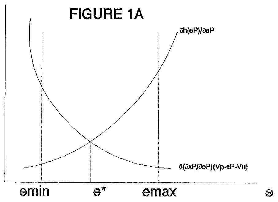
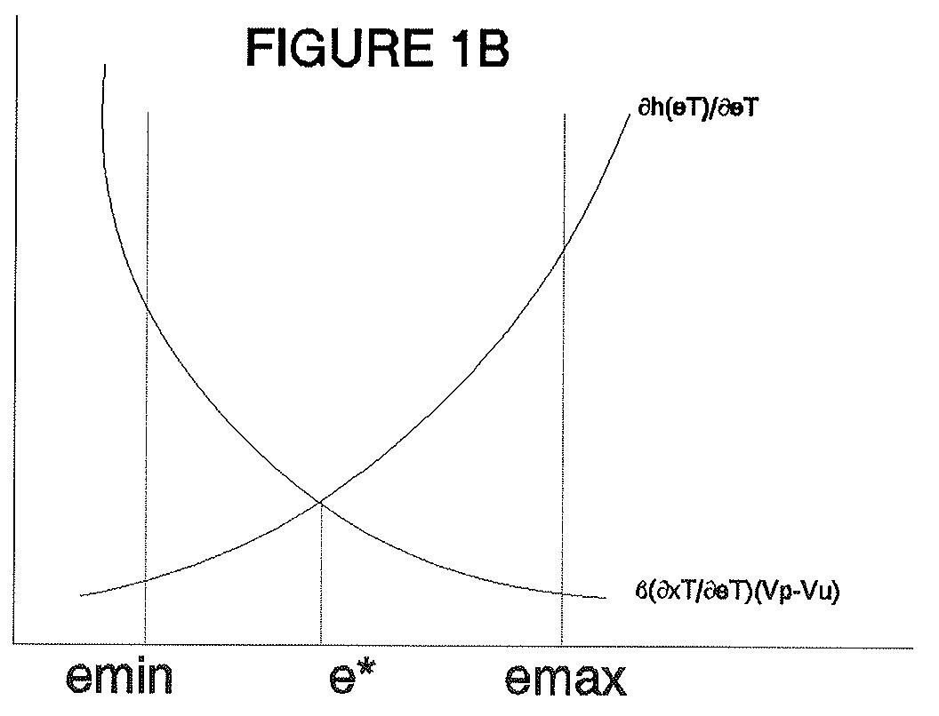
FIGURE 2
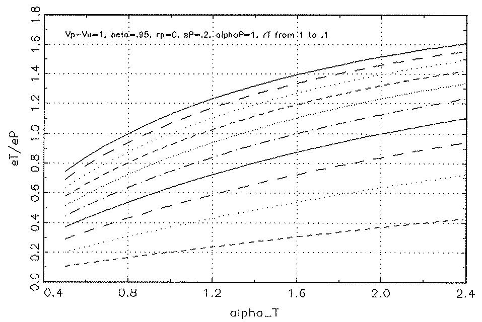
FIGURE 3
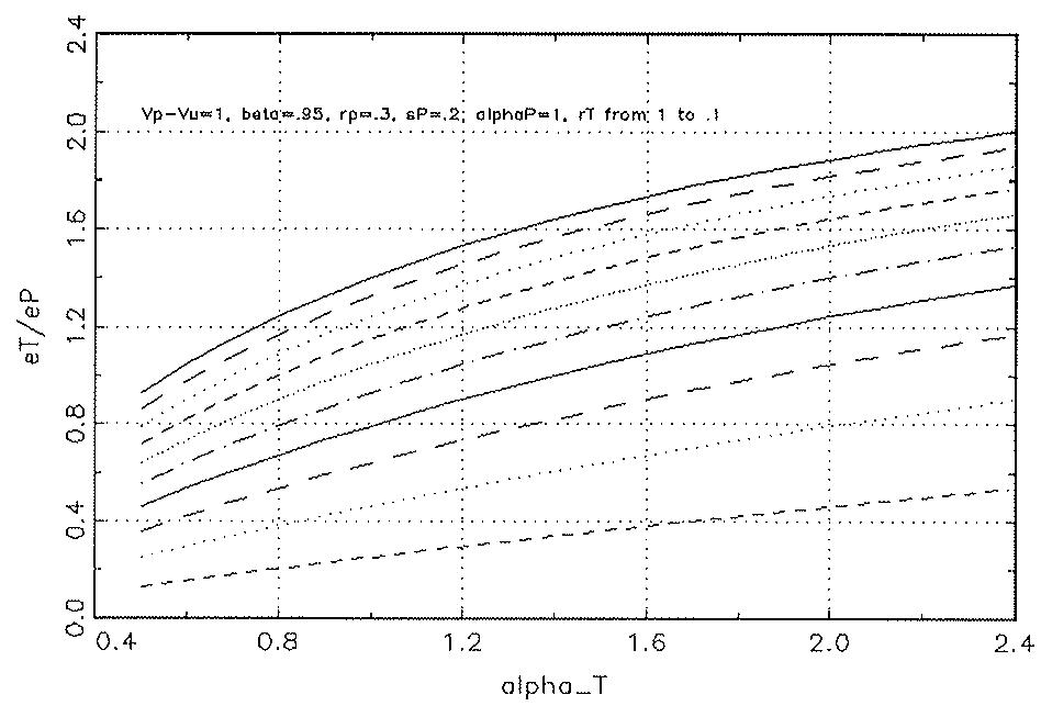
FIGURE 4
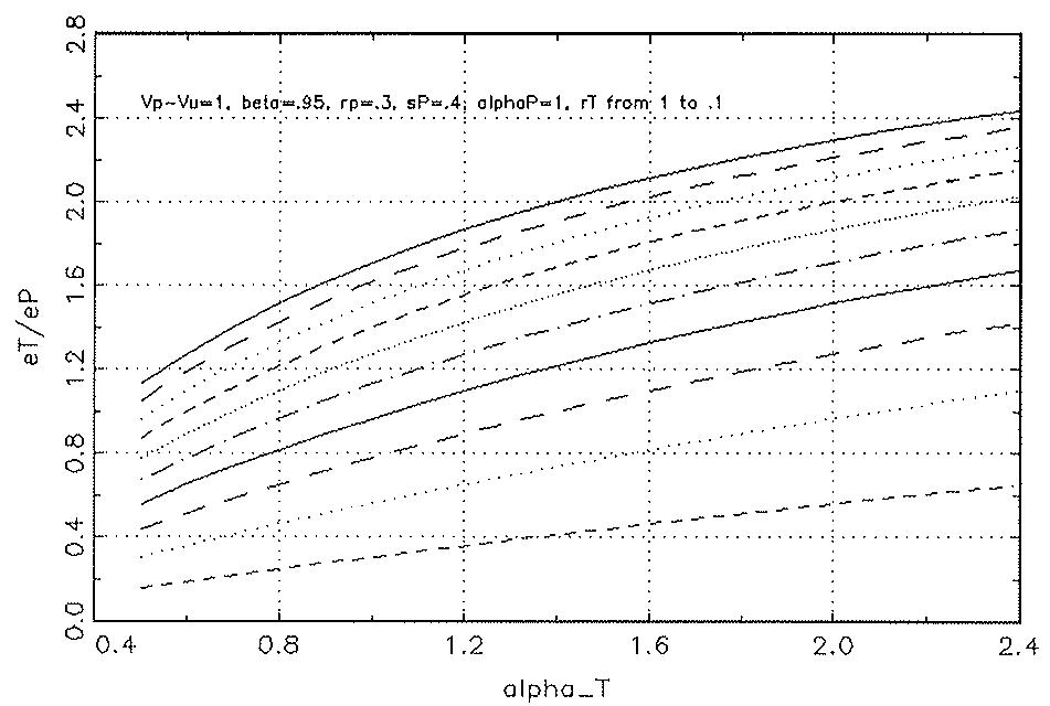
FIGURE 5
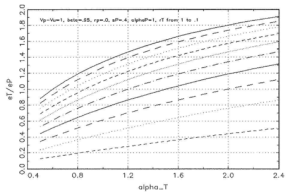
Este texto se ha extraído automáticamente del documento original. Para citarlo o leerlo con su maquetación, descargue el PDF.
Descargar en PDF