THE DETERMINANTS OF LABOUR MOBILITY IN SPAIN: WHO ARE THE MIGRANTS?* by Luis Albériko Gil** and Juan F. Jimeno*** Documento de Trabajo 93-05
May 1993
* We wish to thank Samuel Bentolila, Olympia Bover and Juan J. Dolado for helpful comments. The usual disclaimer applies.
** London School of Economics
*** Universidad de Alcalá de Henares and FEDEA
ABSTRACT
This paper analyses the reasons of the drastic decrease and change in the patterns of inter-regional migration flows in Spain. In principle, inter-regional labour mobility should take place as a response to unemployment and wage differentials across regions and, hence, there are several explanations for low labour mobility. Concretely, in the Spanish case, some interesting developments that should be take into account are: i) an extension of the social protection system that provides to unemployed individuals with alternatives to migration, ii) an increase in mobility cots and cost of living (mainly housing prices) in the low unemployment-high wage regions which, together with a reduction in unemployment and wage differentials, reduce the returns to migration, and iii) a reduction in the employment opportunities (for a given unemployment rate) in the destination regions. To offer some evidence on the ultimate reasons for the observed low inter-regional labour mobility in Spain, we use cross-sectional data from the Labour Force Survey to estimate the probability of moving conditioned on personal characteristics and to observe the employment status of migrants. Our results suggest that an inefficient matching of unemployed and vacancies located in different regions is an important factor behind low labour mobility and, therefore, the improvement of this matching process should be a goal of any employment policy aimed at increasing labour mobility.
JEL Codes: J60, J61
1.- Introduction
Migration flows in Spain have substantially fallen since the 1960s. Nowadays, not only the proportion of migrants is rather low, but also labour mobility does not seem to be taking place as a response to regional unemployment and wage differentials. Some authors (notably, Bentolila and Blanchard (1991)) have argued that these facts are producing a mismatch between labour demand and supply, a problem which is at the heart of high and persistent Spanish unemployment. Hence, an increase in labour mobility is often advocated as a solution to the Spanish unemployment problem. Employment policies aimed at achieving such increase should rely on the identification of the reasons hindering labour mobility. The purpose of this paper is to offer some evidence on the characteristics and determinants of Spanish inter-regional labour mobility.
There are at least two competing theories of labour migration, that we shall label the human capital and the matching theories. According, to the human capital theory of labour migration, individuals migrate to the region where their expected utility, which depends on real wages and the probability of being unemployed, is higher. In particular, they migrate independently of (and, plausibly, before) having found a job in the destination region. Hence, we should observe migration flows from low wage-high unemployment to high wage-low unemployment regions and the reasons for low labour mobility must be found either in low wage and unemployment differentials (maybe, because the perverse effect of a too generous unemployment benefit system and/or relatively higher housing prices in the candidates for destination regions), or in the difference in amenities between regions, or in significant mobility costs.
On the contrary, the matching theory stresses that labour mobility is not intrinsically different from the matching problem between unemployment and job vacancies, with the only difference that some of the unemployed and job vacancies are located in different regions and, in this case, matching is less likely. An obvious implication of this theory is that individuals migrate only after having found a job in a region other than their initial residence region. Hence, the reasons for low labour mobility must be related to the characteristics of the matching process between unemployed and vacancies, and the differences across regions in this matching process. Under this view the employment status of individuals is very relevant to the migration decision, while under the human capital theory of migration (which stresses the expected wage as driving variable of migration) this employment status is less decisive.
Which of the two competing theories is better-suited to explain labour migration is not only an academic issue. Assuming that increasing labour mobility may contribute to reduce unemployment, several employment policies may be recommended to achieve such increase but which one of them is most successful obviously depends on the ultimate reasons hindering labour mobility, which are different under the human capital theory and under the matching theory of migration.
Previous analysis of labour migrations can be classified according to the nature of the data used (time series or cross-sectional data). As examples, one of the most recent studies regarding Spain is Bentolila and Dolado (1990), who following the human capital theory of migration, regress (net) inter regional migration flows on some regional economic variables (wage and unemployment) to find that the response of these flows to real wages and unemployment differentials, is low and slow. On the other hand, Jackman and Savouri (1990) adopt the matching theory and use the British annual data on (gross) inter regional migration in the period 1975-87 to show that regional characteristics, the levels of unemployment (at the regional and national level), the share of long-term unemployment, the mortgage interest rate, distance (plausibly related to information asymmetries) and vacancy rates help to explain these flows. Juárez-Mulero (1991) presents a similar analysis using Spanish data. On the other hand, Antolín and Bover (1993) and Pissarides and Wadsworth (1989) have recently used cross-sectional data to estimate moving probabilities (conditioned on personal characteristics) in Spain and Britain, respectively, and to analyze how regional economic variables affect these moving probabilities.
In this paper, we use a theoretical framework that attempts to capture both the human capital view and the matching view of the migration decision. We present this theoretical framework in section 2 and show that migration without employment (according to the human capital theory) is likely when unemployment and wage differentials are pretty large but that the matching view of migration is more appropriate for lower (an more plausible) inter-regional wage and unemployment differentials. Hence, it could be expected that low labour mobility is a result of an inefficient inter-regional matching process. However, lack of information on the inter-regional matches of unemployed and vacancies precludes a robust empirical assessment of this latter conclusion. We try to substitute this lack of information, analyzing cross-sectional data on the personal characteristics and employment status of migrants and non-migrants, in section 3. After presenting estimates of the moving probability (conditioned on several personal characteristics) we conclude that the matching view of labour migration is very relevant to the Spanish case. Some concluding remarks are in section 4.
Earlier studies using either time series data or cross-sectional data on migration flows are referenced in the papers cited in the text.
Antolín and Bover pool cross-sections of five years (1987-91) of the Spanish Labour Force Survey.
2.- A model of migration
In this section we try to identify the main variables affecting the migration decision. For simplicity, we assume two regions, the origin region (O) and the destination region (D). Residents in O must decide whether or not to move to D, taking into account (real) wages in each region , the frequency and duration of unemployment spells which relate to hiring and firing probabilities , altogether with the one time loss caused by mobility costs (m). We denote by the probability of being hired in region j (O or D) while living in region i (O or D). This dependence of the hiring probabilities on the region of residence is a simple way to capture the matching component of the labour migration decision, altogether with unemployment differentials across regions. For simplicity, we will assume that individuals are risk-neutral.
Real wages are net of unemployment benefits and include the value of amenities if these differ by regions.
We define as the value function of being in the region i in employment status s (unemployed, U, or employed, E). To denote the time discount factor we shall use . We assume that people receive one-job-offer per period of time (at the end of such period) only when they are unemployed. Hence,
\[\begin{array}{c} {V _ {O} ^ {U} = \delta h _ {O} ^ {O}. \max \Bigl \{V _ {O} ^ {U}, V _ {O} ^ {E}, V _ {D} ^ {U} - m \Bigr \} +} \\ \\ {+ \delta \Bigl [ h _ {O} ^ {D}. \max \Bigl \{V _ {O} ^ {U}, V _ {D} ^ {E} - m, V _ {D} ^ {U} - m \Bigr \} + (1 - h _ {O} ^ {O} - h _ {O} ^ {D}). \max \Bigl \{V _ {O} ^ {U}, V _ {D} ^ {U} - m \Bigr \} \Bigr ]} \end{array}\tag{1}\]
\[V _ {O} ^ {E} = w _ {O} + \delta \left[ f. \max \left\{V _ {O} ^ {U}, V _ {D} ^ {U} - m \right\} + (1 - f). \max \left\{V _ {O} ^ {U}, V _ {O} ^ {E}, V _ {D} ^ {U} - m \right\} \right]\tag{2}\]
\[\begin{array}{r l} V _ {D} ^ {U} & = \delta h _ {D} ^ {D}. \max \left\{V _ {O} ^ {U} - m, V _ {D} ^ {U}, V _ {D} ^ {E} \right\} + \\ & + \delta \left[ \bar {h} _ {D} ^ {O}. \max \left\{V _ {O} ^ {U} - m, V _ {D} ^ {U}, V _ {O} ^ {E} - m \right\} + (1 - h _ {D} ^ {D} - h _ {D} ^ {O}). \max \left\{V _ {O} ^ {U} - m, V _ {D} ^ {U} \right\} \right] \end{array}\tag{3}\]
Note, however, that under certain conditions a risk premium can be added to the mobility cost and, thus, our results can encompass certain forms of risk-aversion.
This is for the sake of simplicity and without loss of generality.
\[V _ {D} ^ {E} = w _ {D} + \delta [ f. \max \left\{V _ {D} ^ {U}, V _ {O} ^ {U} - m \right\} + (1 - f). \max \left\{V _ {D} ^ {E}, V _ {D} ^ {U}, V _ {O} ^ {U} - m \right\} ]\tag{4}\]
where, for ease in notation we have assumed that the firing probability, , is invariant across regions. An unemployed person at the origin region receives some unemployment benefit each period (which is normalized to zero) and has several option in the following period depending on whether or not she receives a job offer. In the case she receives a job offer in the origin region, she may choose between accepting the offer, remaining unemployed or moving to be unemployed at the other (destination) region. Alternatively, she may receive a job offer from another (destination) region and, thus, she may choose between accepting the offer, remaining unemployed in the origin region or moving to the other region without accepting the job offer. Finally, when no job offer is received, she may choose between remaining unemployed at the origin region or moving to the other region. Hence, the value to be unemployed at the origin region can be written as in equation (1) above. (Equation (3) is obtained in a similar fashion). An employed person at the origin region receives the corresponding wage and has several options next period depending on whether or not she is fired. If she is not fired, she may choose between remaining employed, quitting the job and becoming unemployed, and quitting the job and moving to another region. If she is fired, she may only choose between the last two of the previous alternatives. Thus, equation (2) represents the value of being employed at the origin region (and, similarly, equation (4) represents the value of being employed in the destination region).
The individual will choose her residence and employment status depending on which of these value functions is higher. We emphasize that this way of setting up the migration decision is within the spirit of the human capital theory. However, by making the hiring probabilities in either region dependent on the region of residence, we capture the matching component of the migration decision and we can ascertain how the current employment status and employment opportunities influence the migration decision. Since we want to focus on the migration decision, we will assume that, within each region, the value of being employed is higher that the value of being unemployed (otherwise, whether to migrate is not an issue). Thus,
\[V _ {O} ^ {E} > V _ {O} ^ {U} \quad a n d \quad V _ {D} ^ {E} > V _ {D} ^ {U}\tag{5}\]
After having defined these value functions, we can obtain the conditions under which labour migration takes place. For instance, when
\[V _ {D} ^ {U} - m > V _ {O} ^ {U}\tag{6}\]
unemployed will migrate to another region even before finding a job in the destination region D (migration without employment). A second possibility is that
It must be noticed that migrations can be permanent or transitory, depending on whether
\[V _ {D} ^ {U} - m < V _ {O} ^ {U} < V _ {D} ^ {E} - m\tag{7}\]
and, in this case, individuals will migrate only after finding a job in the destination region (migration with employment). Finally, no migration takes place when the previous inequality is reversed, that is
\[V _ {O} ^ {U} > V _ {D} ^ {E} - m\tag{8}\]
We will now obtain the parameter values for which, alternatively, no migration, migration without employment and migration with employment take place. Having done this, we can discuss how changes in the parameter values affect the likelihood of migration.
2.1.- Absence of migration
In the case in which no migration takes place, the value functions boil down to:
\[V _ {O} ^ {U} = \delta \left[ h _ {O} ^ {O} V _ {O} ^ {E} + \left(1 - h _ {O} ^ {O}\right) V _ {O} ^ {U} \right]\tag{9}\]
\[V _ {D} ^ {U} = \delta \left[ h _ {D} ^ {D} V _ {D} ^ {E} + \left(1 - h _ {D} ^ {D}\right) V _ {D} ^ {U} \right]\tag{10}\]
and transitory if
Migration with employment is permanent if
\[V _ {O} ^ {E} = w _ {O} + \delta \left[ f V _ {O} ^ {U} + (1 - f) V _ {O} ^ {E} \right]\tag{11}\]
\[V _ {D} ^ {E} = w _ {D} + \delta \left[ f V _ {D} ^ {U} + (1 - f) V _ {D} ^ {E} \right]\tag{12}\]
and, after some manipulation:
\[V _ {O} ^ {E} = \frac {w _ {O} \left[ 1 - \delta \left(1 - h _ {O} ^ {O}\right) \right]}{(1 - \delta) \left[ 1 - \delta \left(1 - f - h _ {O} ^ {O}\right) \right]}\tag{13}\]
\[V _ {O} ^ {U} = \frac {\delta h _ {O} ^ {O} w _ {O}}{(1 - \delta) [ 1 - \delta (1 - f - h _ {O} ^ {O}) ]}\tag{14}\]
\[V _ {D} ^ {E} = \frac {w _ {D} \left[ 1 - \delta \left(1 - h _ {D} ^ {D}\right) \right]}{(1 - \delta) \left[ 1 - \delta \left(1 - f - h _ {D} ^ {D}\right) \right]}\tag{15}\]
\[V _ {D} ^ {U} = \frac {\delta h _ {D} ^ {D} w _ {D}}{(1 - \delta) [ 1 - \delta (1 - f - h _ {D} ^ {D}) ]}\tag{16}\]
and, thus, the condition under which migration does not take place, , is equivalent to
\[\frac {\delta h _ {O} ^ {O} w _ {O}}{1 - \delta (1 - f - h _ {O} ^ {O})} > \frac {w _ {D} [ 1 - \delta (1 - h _ {D} ^ {D}) ]}{1 - \delta (1 - f - h _ {D} ^ {D})} - (1 - \delta) m\tag{17}\]
Hence, high mobility costs, high wages in the origin region, low alternative wages in other regions, high hiring rates in the origin region, low hiring rates in the destination region and high firing rates, make this inequality more likely to hold and, thus, may be among the reasons of non-existent inter-regional labour mobility.
2.2. Migration with and without employment
At the other extreme, it could be the case that workers migrate with or without employment. In the case of migration without employment (i.e., moving into unemployment in the destination region), the value functions become
\[V _ {O} ^ {U} = \delta \left[ h _ {O} ^ {O} V _ {O} ^ {E} + h _ {O} ^ {D} (V _ {D} ^ {E} - m) + (1 - h _ {O} ^ {O} - h _ {O} ^ {D}) (V _ {D} ^ {U} - m) \right]\tag{18}\]
\[V _ {O} ^ {E} = w _ {O} + \delta [ f (V _ {D} ^ {U} - m) + (1 - f) V _ {O} ^ {E} ]\tag{19}\]
\[V _ {D} ^ {U} = \delta \left[ h _ {D} ^ {D} V _ {D} ^ {E} + (1 - h _ {D} ^ {D}) V _ {D} ^ {U} \right]\tag{20}\]
\[V _ {D} ^ {E} = w _ {D} + \delta [ (1 - f) V _ {D} ^ {E} + f V _ {D} ^ {U} ]\tag{21}\]
and after some manipulation:
\[V _ {D} ^ {U} = \frac {\delta h _ {D} ^ {D} w _ {D}}{(1 - \delta) [ 1 - \delta (1 - f - h _ {D} ^ {D}) ]}\tag{22}\]
\[V _ {D} ^ {E} = \frac {w _ {D} [ 1 - \delta (1 - h _ {D} ^ {D}) ]}{(1 - \delta) [ 1 - \delta (1 - f - h _ {D} ^ {D}) ]}\tag{23}\]
\[V _ {O} ^ {E} = \frac {(1 - \delta) [ 1 - \delta (1 - f - h _ {D} ^ {D}) ] (w _ {O} - \delta f m) + \delta^ {2} f h _ {D} ^ {D} w _ {D}}{(1 - \delta) [ 1 - \delta (1 - f - h _ {D} ^ {D}) ] [ 1 - \delta (1 - f) ]}\tag{24}\]
\[V _ {O} ^ {U} = \frac {\delta \left[ h _ {O} ^ {O} w _ {O} + h _ {O} ^ {D} w _ {D} - (1 - \delta) h _ {O} ^ {D} m \right]}{1 - \delta (1 - f)} +\tag{25}\]
\[+ \frac {\delta (1 - \delta) \left(1 - h _ {O} ^ {O} - h _ {O} ^ {D}\right) + \delta^ {2} f}{1 - \delta (1 - f)} \left[ \frac {\delta h _ {D} ^ {D} w _ {D}}{(1 - \delta) [ 1 - \delta (1 - f - h _ {D} ^ {D}) ]} - m \right]\]
Therefore, the condition under which unemployed will move to another regions even before finding a job is given by:
\[\left(\frac {\delta h _ {D} ^ {D} w _ {D}}{1 - \delta (1 - f - h _ {D} ^ {D})} - (1 - \delta) m\right) > \frac {\delta [ h _ {O} ^ {O} w _ {O} + h _ {O} ^ {D} w _ {D} - (1 - \delta) h _ {O} ^ {D} m ]}{1 - \delta (1 - f - h _ {O} ^ {O} - h _ {O} ^ {D})}\tag{26}\]
Consequently, low mobility costs, low wages in the origin region, high alternative wages in other regions, low hiring rates in the origin region, high hiring rates in the destination region and low firing rates, make this inequality more likely to hold and, thus, promote labour mobility. It must also be noticed than an increase in the probability of receiving a job offer from another region without leaving the origin region ( ), reduces the likelihood of migration without employment.
Hence, inequalities (17) and (26) define three different regimes regarding labour mobility. When inequality (17) is satisfied, no migration takes place, even if individuals receive job offers from other regions. In this regime, only an increase in wage and unemployment differentials across regions or a reduction in mobility costs can promote labour mobility. When inequality (26) is satisfied, there will be migrants moving without jobs. When neither of inequalities (17) and (26) is satisfied, individuals will migrate only after receiving a job offer in the destination region. In this latter regime, the main restriction to labour mobility is the matching between unemployed and vacancies located in different regions, although, as in the no migration case, a sufficient increase in wage and unemployment differentials and a reduction in mobility costs can promote labour mobility (by switching regimes to the migration without employment regime). It must be noticed that when the probability of receiving a job offer from another region while living at the origin region, , is nil (an implicit assumption in the human capital theory of migration) then inequalities (17) and (26) are equivalent and, thus, we can focus only on two regimes: absence of migration and migration without employment (since migration with employment is not feasible). Alternatively, the closer this probability is to the hiring rate at the destination region, , the more likely is that migration takes place only with employment, since there is no gain from moving (and paying a positive mobility cost) before receiving a job offer in the destination region. In this case, the matching component of migration is most relevant since only migration with employment will take place (as long as mobility costs are positive).
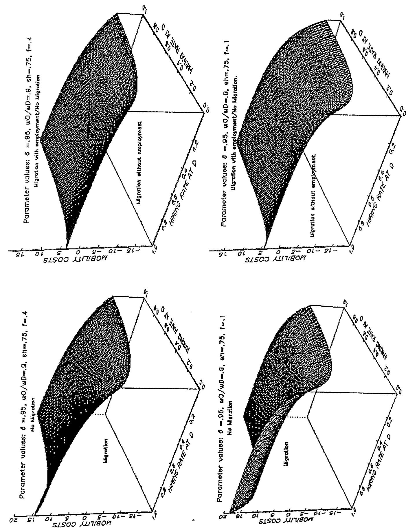
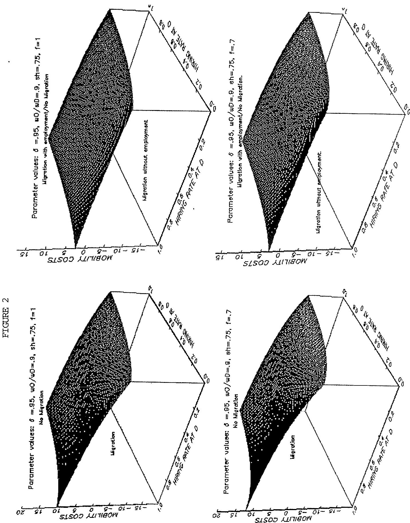
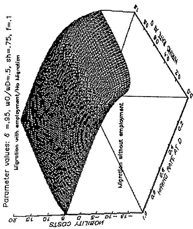
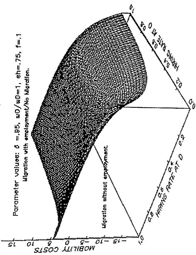
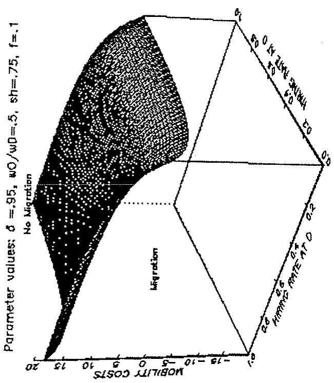
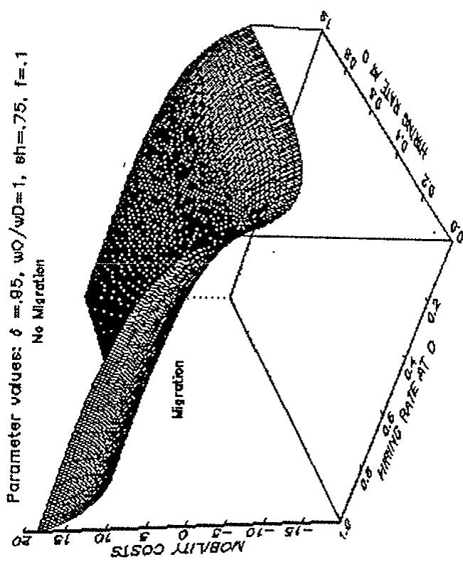
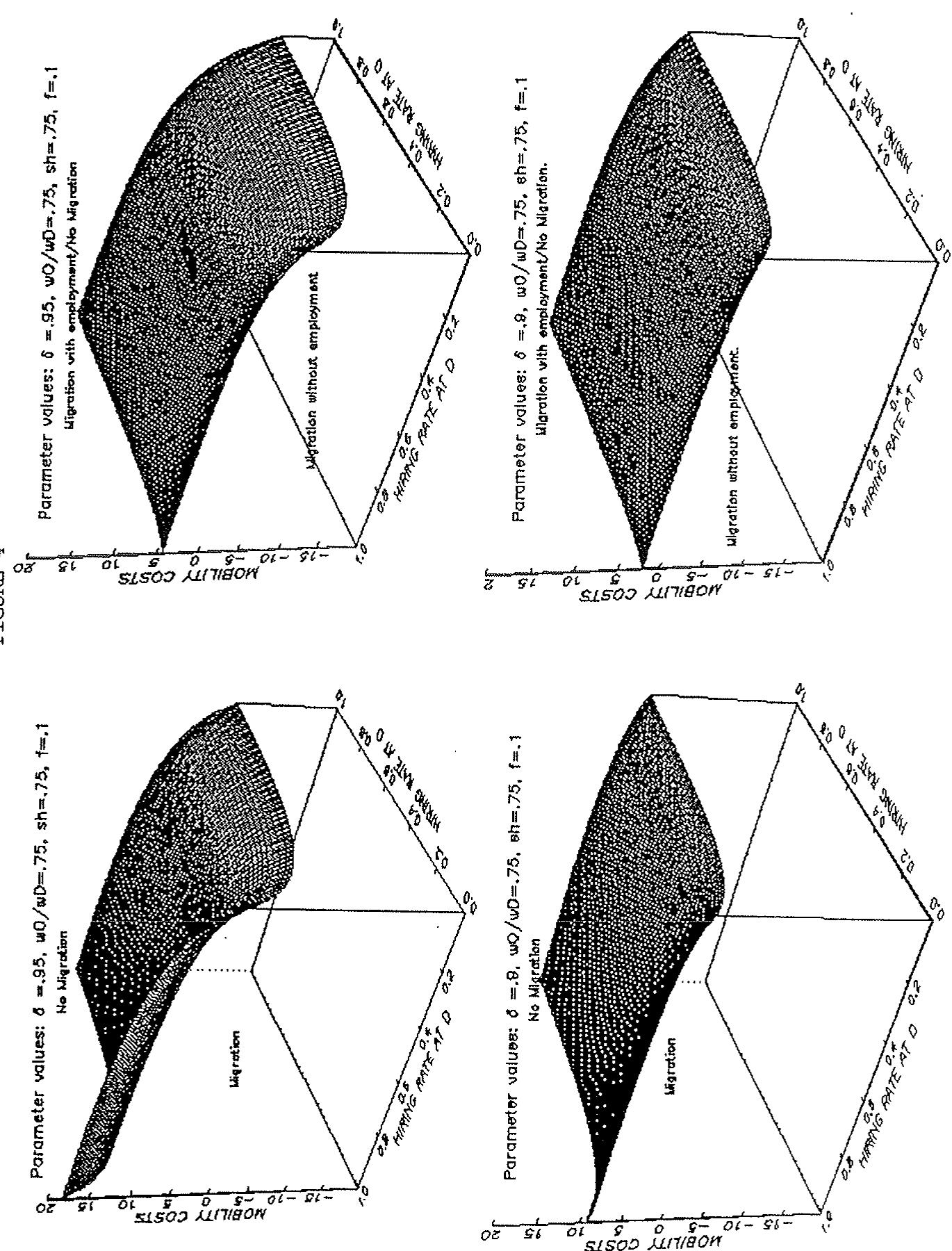
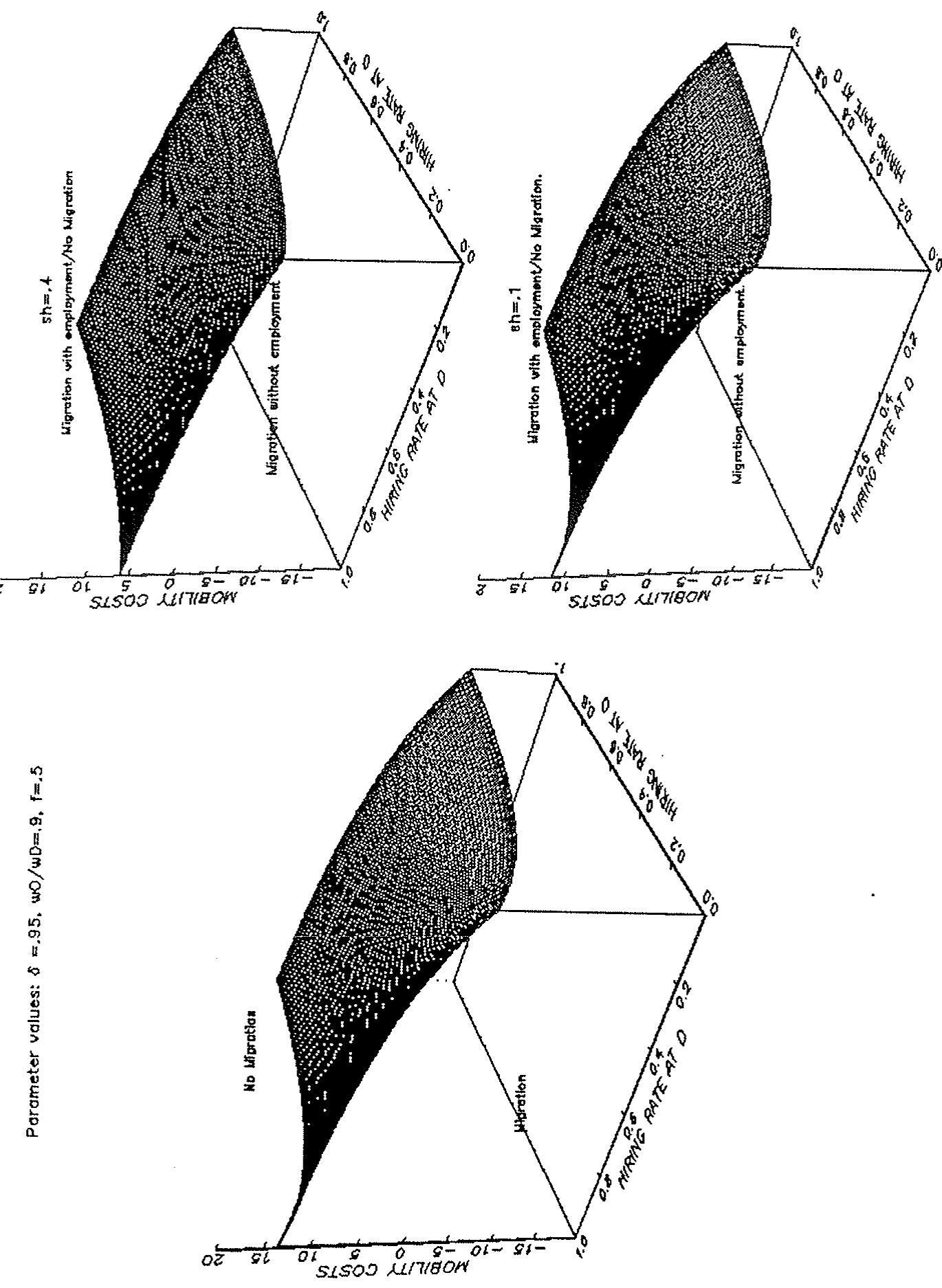
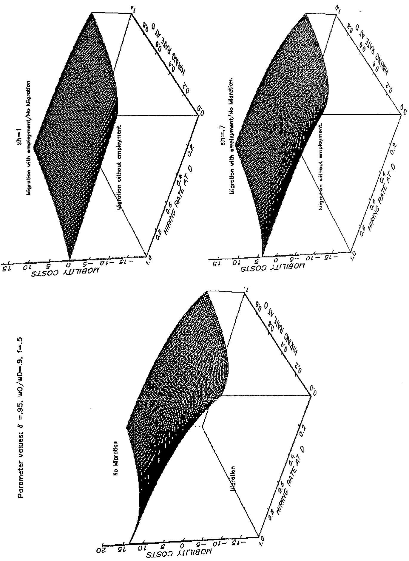
To get some feeling on the relative importance of the several determinants of migration in each one of these regimes and on which regime is most likely for plausible parameter values, we perform some simulations. The results of these simulations are plotted in figures 1 to 6. These figures represent the ranges of hiring probabilities at the origin and destination regions, and , and of mobility costs (normalized by the wage in the destination region, ) for which each one of the three possibilities analyzed (no migration, migration without employment and migration with employment) arise, given different sets of the parameter values, , -normalized by , and , the latter being the ratio of the probability of finding a job in the destination region before moving to that probability after moving, . These figures are always drawn on the same scale so that they can be easily compared.
Several interesting facts are illustrated by these figures. The range of values of mobility costs for which migration (with and without employment) takes place is obviously increasing with the hiring rate at the destination region and decreasing with the hiring rate at the origin region. More interestingly, figures 1 and 2 show how changes in the firing rate affects the migration decision. A firing rate equal to one (up-left panel of figure 2) reduces substantially the range of values of mobility costs for which migration takes place (see, for instance, the bottom-left panel of figure 1 where the firing rate is only 0.1).
Firing rates are relevant to the Spanish case where the average job tenure has dramatically fallen as a consequence of the increasing incidence of fixed-term employment contracts. In 1984 the Spanish government introduced several legal reforms to increase the flexibility of the labour market. These reforms
Figures 3 and 4 show the effects of different wage differentials and discount factors. Wage differentials play an important role in the migration decision when hiring probabilities in both regions are high enough. Otherwise, the change in the mobility costs which make the individual indifferent between migrate or not is not remarkable. The same can be said for the comparison of the decision between migration with and without employment. An increase in the discount factor (figure 4) makes migration more likely (as could be expected for appropriate values of the rest of the parameters). Finally, figures 5 and 6 present how the ratio of the hiring rate at the destination region when living at the origin region to that hiring rate after moving, affects the range of value of mobility costs for which migration without employment takes place. Obviously, when this ratio is close to one, migration without employment requires very low (even negative) mobility costs. When this ratio is close to zero, migration with employment is barely feasible and, hence, all migration is without employment. In the former case, low labour mobility is a consequence of a low hiring rate at the destination region.
consisted of liberalising the use of fixed-term employment contracts, somehow restricted before that date. Since then, fixed-term employment in Spain has increased from about 10% at the beginning of 1985 up to more than 30%, currently (see Segura et. al. (1991)). The employment effects of these reforms have been analyzed by Bentolila and Saint-Paul (1992). Plausible productivity and wage effects of fixed-term employment have been shown by Jimeno and Toharia (1993) and Dolado and Bentolila (1992).
3.- Personal characteristics and employment status of migrants
In this section we first estimate moving probabilities using information from the Spanish Labour Force Survey (second quarter of 1991). Our final goal is to establish the reasons for the observed low inter-regional labour mobility. We, however, cannot observe whether migrants move before or only after having found a job in the destination region. Thus, as an attempt to identify the reasons for the low labour mobility observed, we also estimate the effects of the migration decision on the current employment status and infer from these effects the changes in the employment status of migrants and non-migrants. The use of cross-sectional data allows us to control for a wide range of personal characteristics that introduce composition effects which complicate the analysis of aggregate time series data on migration flows and inter-regional unemployment and wage differentials.
A.- Who are the migrants?
The empirical implementation of the model presented in section 2 using cross-sectional data can be performed with the following
The Spanish Labour Force Survey contains, but only on the second quarter of each year, a question about the place of residence and employment status of individuals one year earlier. We define migrants as those people who declare a different region of residence one year earlier than that at the date of the survey. We choose the second quarter of 1991 because, precisely together with the Labour Force Survey of the second quarter of 1990, an experimental survey on earnings was carried out, so that for that date we can estimate wage differentials conditioned on some personal characteristics. Antolín and Bover (1993) have estimated moving probabilities using similar data but pooling information for five years (1987-91).
specification:
\[y = 0, \text { if } V _ {O} ^ {U} > V _ {D} ^ {E} - m (\text { condition (17) holds })\]
\[y = 1, \text { if } V _ {D} ^ {E} - m > V _ {O} ^ {U} > V _ {D} ^ {U} - m \text {(conditions (17) and (26) do not hold)}\]
\[y = 2, \text { if } V _ {D} ^ {U} - m > V _ {O} ^ {U} (\text { conditions (17) do not hold and (26) holds })\]
where the values of y (0,1,2) represent no migration, migration (only) with employment and migration without employment, respectively. Thus, this model can be casted in a multinomial (logit) probit specification, which could be estimated by maximum-likelihood in cross-section samples of individuals.
However, there are some difficulties in this approach related to the non-observability in most available samples of the variables that determine the value functions and of the type of migration. In our sample (taken from the Spanish Labour Force Survey), we observe workers who declare that their current place of residence is different from that one year earlier, so we can identify "migrants/movers" (in this restrictive sense). Unfortunately, we cannot know if the workers who migrated did it before or after having found a job in the destination region. Thus, in principle, the econometric specification above cannot be directly estimated. Secondly, wage differentials, individual-specific hiring and firing probabilities and mobility costs are not directly observed either. Nevertheless, we can use personal characteristics of the workers to proxy for those variables (and, in this regard, the Labour Force Survey offers a wide variety of choices). Thus, we first estimate the following (binomial) probit model:
Note, however, that we have no information about temporary migration of less than one year of duration.
\[p = \text { Prob } [ y = 0, (\text { No migration }) ] = \text { Prob } [ V _ {O} ^ {U} - V _ {D} ^ {E} + m > 0 ] = f (X ^ {\prime} \beta)\]
\[\text {Prob} [ y = 1 \text {or} y = 2, (\text {Migration}) ] = \text {Prob} [ V _ {O} ^ {U} - V _ {D} ^ {E} - m < 0 ] = 1 - p\]
where X is a vector of individual characteristics, is a vector of parameters and f a cumulative (normal) distribution function.
Before discussing the results obtained from this estimation, several comments ought to be made:
i) The sample contains individuals (male and female) who were either employed or unemployed in the second quarter of 1991 (so we have excluded those people not in the labour force at that date). Some information on sample composition is in Table 1. It has been argued that females have a different behaviour that males when taking migration decisions since they are more likely to be "tied movers" (see, for instance, Antolín and Bover (1993)). Additionally, individuals who were out of the labour force one year earlier and currently participate in the labour market, are individuals who jointly decided about migration and participating in the labour market. We also split up the sample in two sub-samples: employed and unemployed one year earlier to the reference period of the sample. This is done for two reasons: first, to eliminate the problem of the joint decision on participation and migration that the inclusion in the sample of individuals out of the labour one year earlier introduces in the interpretation of the estimates of moving probabilities on the whole sample, and, secondly, since the employment status prior to the migration decision is very likely to affect such decision (see section 2), it is convenient to estimate the moving probabilities of these two groups of individuals separately. In our sample the number of migrants is very low, so that the estimates from both the whole sample and the two sub-samples cited above have, in general, large standard errors. Antolín and Bover (1993) pool five years of the Spanish Labour Force Survey and estimate moving probabilities from a sample with a much larger number of observations, although the proportion of migrants in that sample is very similar to that in our sample (about 0.3 %).
ii) We have identified migrants as individuals with different places of residence between the second quarter of 1990 and the second quarter of 1991, where place of residence is one of the following groups of regions:
a) Northwest (Galicia, Asturias, Cantabria)
b) Northeast (Basque Country, Navarra, Rioja, Aragon)
c) Madrid
d) Center (Castilla-Leon, Castilla-La Mancha, Extremadura)
e) East (Catalonia, Valencia, Balearic Islands),
f) South (Andalucia, Murcia, Ceuta, Melilla),
g) Canary Islands.
Among these regions, the South, the Center and Canary Islands have the highest unemployment rate (in the 20-25% range in 1990). The regions with higher average wages are the Northeast, Madrid and the East.
iii) The percentage of migrants (between the groups of regions above) in this sample is surprisingly low, a mere 0.3% (270 out of 77,394 in the sample). This low figure raises questions about the efficiency of the Spanish Labour Force Survey at measuring inter-regional labour migration flows. (However, the information obtained by this survey is used to compute Spanish official statistics on migration that lead researchers to assess the huge decrease in labour migrations observed in Spain, as already commented in the introduction. For instance, according to these official statistics, total inter-regional migrations -not only, labour migrations- accounted for .48% of total population (INE (1991)). Our estimates of moving probabilities are conditioned on a set of variables that plausibly are equally distributed both in the population and in the sample of the Labour Force Survey.
iv) Most of the personal characteristics of the workers that we observe are those of the reference period of the survey (the second quarter of 1991). In fact, the survey only offers information as of one year earlier on the employment status (not in the labour force, employed or unemployed) and broad occupation (employer, "family-helper", wage-earner in the public sector, wage-earner in the private sector). It is obvious that some of those personal characteristics are either invariant or variant in a predictable way (like sex and age, for instance).
However, variables referring to family relations (household, wife/husband of household, relative of household, non-relative of household) and marital status (married or non-married) are likely to change as a consequence of migration. This must be taken into account when interpreting the results.
The results, presented in Table 2, show that not only moving probabilities (100 minus the probabilities reported in Table 2) are low, but that they are so for most individuals. In the third column of table 2, we report the moving probabilities estimated on the whole sample (individuals currently participating in the labour market but not necessarily so one year earlier). These probabilities confirm that moving probabilities increase with levels of education and decrease with age (although not all of the corresponding coefficients are statistically significant). Males and married people are also more likely to move (although it must be remembered than the civil status is that posterior to the migration and may be a consequence rather than a cause) while individuals with children are less likely to migrate, especially when these children are 7-16 years old. With regard to the origin region, the differences, with the exception of Madrid and the Northwest, are not remarkably large. More interestingly, individuals unemployed one year earlier are less likely to move than those either employed or out of the labour force at the same date. This finding that seems counterintuitive is often present in studies with cross-sectional individual data (see, for instance, Pissarides and Wadsworth (1991) and Antolín and Bover (1993)). As commented above, it may be due to the inclusion of individuals who jointly decide on participating in the labour market and migrating (those out of the labour force) and to the imposition of the restriction that the effect of the employment status prior to the migration decision can be captured by a dummy variable without differences in the rest of the parameters of the model.
In columns (1) and (2) of Table 2, we present the moving probabilities estimated from two different groups of the sample, individuals employed one year earlier and those unemployed at the same date. Once the restriction imposed on the estimation reported in column (3) of the same table is relaxed, we find that the unemployed are more likely to migrate than the employed (with minor exceptions regarding youths without studies). Regarding personal characteristics, their influence on the migration decision is of the same sign than that found in the whole sample (although the magnitude of the coefficients changes). It is also interesting that the regional dummies estimated on the two subsamples show the same pattern of migration flows than that in the whole sample, with Madrid and the Northwest being the origin regions with larger moving probabilities and the South, the Northeast and the Center being those with smaller moving probabilities. These results are especially remarkable since, in principle, migration flows from low wages-high unemployment regions to high wage-low unemployment regions should be expected. On this basis, the South and the Center should be among the regions with higher out-migration flows and Madrid and the Northeast should be among those with smaller ones, which is consistent with our results only in the case of the
Northeast.
B. Why is inter-regional labour mobility in Spain so low?.
The results presented in the previous subsection suggest, not only a quantitative decrease, but also a qualitative change in Spanish inter-regional migration flows. Labour mobility is low and, furthermore, the regional patterns of migration flows is different to that which could be expected from a simple human capital model, that is, out-migration from low wage-high unemployment regions (especially, the South and the Center, in the Spanish case). Our theoretical results in section 2 suggest that there are two possible reasons for this situation:
i) The first reason is that regional unemployment and wage differentials are low so that, for plausible mobility costs, individuals are not willing to migrate. In other words, the Spanish economy is in the no migration regime described in section 2. There are, however, several remarks to make. First, average unemployment rates and average wages are not the variables affecting the individual migration decision. What a potential migrant considers when taking her migration decision is her unemployment probability and expected wage in the destination region which may be related to the average values of these variables but also is very likely affected by her personal characteristics. Hence, in the analysis of this issue, unemployment and wage differentials must be computed after eliminating employment composition effects. Secondly, unemployment rates are the result of certain hiring and firing rates so that several combinations of these can yield a given unemployment rate. However, as our results in section 2 show, the migration decision is affected by both hiring and firing rates so that a increase in both that leaves unchanged the unemployment rate does affect the migration decision. In this regard, it is important to bear in mind the huge increase in fixed-term employment in Spain since 1986, which has resulted in significant flows from employment into unemployment and high firing rates for those employed under this type of contracts.
The specification of our model precludes further economic interpretation of the regional differences in moving probabilities. Antolín and Bover (1993) estimate a similar model where regional dummies are substituted by regional economic variables (like unemployment rates, housing prices and average real wages). Their results mainly suggest that subsidies to unemployment is the main reason for low migration flows from low wages-high unemployment regions and that high housing prices is behind high migration flows from high wages-low unemployment regions (especially, Madrid).
ii) The second explanation of low labour mobility could be that most potential migrants are in what we have called migration with employment regime in section 2. In other words, they are willing to migrate and would do so only after receiving a job offer in another region. This possibility arises when the hiring rates in the destination region while living in the origin region is not very different to the hiring rate in the destination region after migration (in the notation of section 2, sh is close to one). In this case, low labour mobility is the consequence of a inefficient matching process that makes both hiring rates at the origin region and at the destination region low.
We now try to assess which of the two previous explanations is closer to the Spanish experience. We face a serious problem: we do not observe the employment status of the migrant immediately previous and immediately after migration took place. In other words, we cannot know if individuals migrate with or without unemployment and, consequently, we cannot conclude if individuals who do not migrate would do so if receiving a job offer from another region. However, we can estimate to what extent the employment status of the individual is affected by migration. Thus, we look at the employment status of the labour force and its relationship with migration controlling for several personal characteristics. We also estimate the probability of holding a permanent employment versus holding a fixed term employment (which implies a much larger firing probability than the former) as a function of personal characteristics and being a migrant or not.
Table 3A and 3B present the employment status of migrants and non-migrants in the current and previous year of the sample. As shown in this table, the incidence of unemployment is higher among migrants than among non-migrants. Furthermore, the (probit) estimates of the probability of being unemployed are substantially higher for migrants, even after controlling for other personal characteristics (see column 3 of table 4). However, after splitting the sample according to the employment status one year earlier, we found that this positive effect of migration on unemployment is present only for those employed one year earlier while individuals unemployed who migrated have a substantially (and significant) lower probability of being unemployed. One plausible interpretation of these results is that those migrants unemployed one year earlier migrated after having found a job and, hence, they are less likely to be unemployed. On the other hand, migration increases the unemployment probability for those migrating without employment (which further discourages labour mobility). There might be several reasons for this: the first possibility is hiring discrimination against migrants; secondly, migrants could be less aware of the local labour market conditions in the destination region than the natives of that region, so that they have a lower probability of finding employment; and thirdly, given the characteristics our definition of migrant, it is conceivable that individuals employed one year earlier also migrate with employment but that they lose it in the interim period, that is, it takes less than one year to find employment in the destination regions, to move and being fired. This latter possibility might sound unrealistic but taking into account the very high employment turnover rate existing in Spain because of the widespread use of fixed-term contract, it may not be so unplausible.
Other interesting conclusions that we can reach from the estimates of probabilities presented in table 4 is that unemployment rates, after controlling for the composition of the labour force, are higher in the South and in the Canary Islands, while in the rest six regions considered the differences are not very large (Of course, the differences in unemployment rates within each region are larger. See for instance Jimeno and Toharia (1993)). There is also a high state-dependence effect: those employed one year earlier are much less likely to be unemployed. With respect to the other variables included, our results confirm those previously obtained by other researchers: unemployment probabilities decrease with levels of education and age, and are higher for females.
Finally, also the type of employment contract significantly differs between migrants and non-migrants. Tables 5 and 6 present the proportion of permanent and fixed term employment contracts for migrants and non-migrants and the (probit) estimates of the probability of being employed under a permanent contract (versus being employed under a fixed term contract), respectively. As can be seen in these tables, the incidence of fixed term employment is much higher among migrants, as could be expected from the fact that migration and entrance into a new job are much related and this entrance is mostly under fixed term employment contracts. However, after splitting the sample according to previous year employment status, we find that migration increases the probability of holding a fixed term employment contracts in the case of unemployed (although the corresponding coefficient is not significantly different from zero), while decreases substantially (and significantly) in the case of employed. These findings are consistent with the existence of positive effects of permanent employment on migration for those who migrate with employment and of negative effects of fixed term employment for those considering migrate without employment.
4.- Concluding Remarks
In this paper, we have analyzed the determinants of labour interregional migrations and have presented some empirical evidence for the Spanish case. We have shown that, for plausible inter-regional wage and unemployment differentials, migration with employment is more likely that migration without employment and that, therefore, the main restriction to labour mobility is a inefficient matching process. After estimating the moving probabilities of different groups of people (defined in terms of several personal characteristics), we have found that these probabilities are low and that they do not differ much among these groups. Moving probabilities are higher for youths, males, and married people without children. To answer why migration flows are so low, we have estimated unemployment rate differentials across regions, controlling for the composition of unemployment. We have found that these differentials are not substantial and, surprisingly, that, in general, migrants have a higher probability of being unemployed than non-migrants, although individuals unemployed prior to migration have reduced their unemployment probability by migrating. Finally, the probability of holding a fixed term job versus holding a permanent job is also higher for migrants, which is not surprising given that fixed term employment contracts is the usual pattern of entry into new jobs, although, again, migrants unemployed one year earlier have higher probability of holding a permanent employment than unemployed-non migrants. These two findings suggest that there is a substantial proportion of migrants who become so after receiving a (permanent) job offer in a different region and, thus, confirm our conjecture on the importance of the lack of an efficient matching process between unemployed and job vacancies located in different regions as a cause of low labour mobility.
References
- Antolín P., and O. Bover (1993): "Regional Migrations in Spain: The Effects of Personal Characteristics, and Unemployment, Wage and House Price Differentials Using Pooled Cross-Sections". Bank of Spain, mimeo.
- Bentolila, S. and O.J. Blanchard (1990): "Spanish unemployment", Economic Policy, 10.
- Bentolila, S. and J.J. Dolado (1990): "Mismatch and Internal Migration in Spain, 1962-86", in F. Padoa-Schiopa, ed., Mismatch and Labour Mobility, London: CEPR.
- Bentolila, S. and G. Saint-Paul (1992): "The Macroeconomic Impact of Flexible Employment Contracts: An Application to Spain", European Economic Review, 36.
- Dolado, J.J. and S. Bentolila (1992): "Who are the insiders?: Wage setting in Spanish manufacturing firms", Bank of Spain, mimeo.
- Instituto Nacional de Estadística, INE, (1991), Encuesta de Población Activa: Encuesta de Migraciones, 1989, Madrid.
- Jackman, R. and S. Savouri (1991): "An Analysis of Migration based on the Hiring Function", University of Oxford, Institute of Economic and Statistics, Applied Economic Discussion Paper Series, no. 98.
- Jimeno, J.F. and L. Toharia (1992): "Productivity and Wage Effect of Fixed-Term Employment Contract: Evidence from Spain", Fundación de Estudios de Economía Aplicada, (FEDEA), working paper no.92-11.
- Jimeno, J.F. and L. Toharia (1993), Unemployment and Labour Market Flexibility: Spain, International Labour Office (forthcoming).
- Juárez-Mulero, J.P. (1991): "Study of the Economic Determinants of Regional Migration Flows: Spain, 1962-85", London School of Economics, mimeo.
- Pissarides, C. and J. Wadsworth (1989): "Unemployment and the Inter-Regional Mobility of Labour", Economic Journal, 99, 739-55.
- Segura, J., F. Durán, L. Toharia and S. Bentolila (1991), Análisis de la Contratación Temporal en España, Madrid: Ministerio de Trabajo y Seguridad Social.
TABLE 1 SAMPLE COMPOSITION
| SAMPLE COMPOSITION | |||
| Non-migrant | 77124 | 99.7% | |
| Migrant | 270 | 0.3% | |
| AGE | 16-18 | 2138 | 2.8% |
| AGE | 19-24 | 12061 | 15.7% |
| AGE | 25-40 | 32439 | 42.2% |
| AGE | 41-55 | 21284 | 27.7% |
| AGE | > 55 | 8911 | 11.6% |
| Without Studies | 7591 | 9.8% | |
| Primary Studies | 47175 | 60.9% | |
| Secondary Studies | 13444 | 17.4% | |
| University | 9184 | 11.8% | |
| Household | 35335 | 45.7% | |
| Wife/Husband of Household | 13469 | 17.4% | |
| Relative of Household | 28009 | 36.2% | |
| Non-Household | 581 | 0.8% | |
| Married | 47827 | 61.8% | |
| Non-Married | 29567 | 38.2% | |
| Employed one year earlier | 58353 | 75.4% | |
| Unemployed one year earlier | 11217 | 14.5% | |
| Inactive one year earlier | 4844 | 6.3% | |
| Male | 49969 | 61.8% | |
| Female | 29567 | 38.2% | |
| Living currently in | |||
| Northwest | 9642 | 12.5% | |
| Northeast | 10895 | 14.1% | |
| Madrid | 3901 | 5.0% | |
| Center | 15948 | 20.6% | |
| East | 17623 | 22.8% | |
| South | 15611 | 20.2% | |
| Canary-Islands | 3712 | 4.8% | |
| With no children 0-6 years old | 64857 | 83.8% | |
| With 1-2 children 0-6 years old | 12379 | 16.0% | |
| With more than 2 children 0-6 years old | 158 | 0.2% | |
| With no children 7-16 years old | 53671 | 69.3% | |
| With 1-2 children 7-16 years old | 21351 | 27.7% | |
| With more than 2 children 7-16 years old | 2272 | 2.9% | |
Reference individuals: Age 16-18, Female, Non-married. Living in Northwest past year, inactive past year, without studies, household. Total Observations: 77,394. Observations with missing values: 561. Sample size: 76,833. Movers: 267. (1) Individuals employed one year earlier. (2) Individuals unemployed one year earlier. (3) All individuals. PROBIT ESTIMATES OF THE PROBABILITY OF LIVING AT THE SAME REGION OF RESIDENCE AS OF ONE YEAR EARLIER D.T. 93-05 por Luis Albériko Gil and Juan F. Jimeno
| VARIABLE | (1) | (2) | (3) | ||||||
| Coefficient | Standard Error | Probability (%) | Coefficient | Standard Error | Probability (%) | Coefficient | Standard Error | Probability (%) | |
| Constant | 2.772 | 0.340 | 99.72 | 2.134 | 0.479 | 98.36 | 2.330 | 0.201 | 99.01 |
| AGE 19-24 | -0.485 | 0.307 | 98.89 | 0.459 | 0.228 | 99.52 | -0.254 | 0.149 | 98.10 |
| AGE 25-40 | -0.497 | 0.305 | 98.85 | 0.400 | 0.232 | 99.44 | -0.257 | 0.150 | 98.09 |
| AGE 41-55 | -0.088 | 0.312 | 99.64 | 0.556 | 0.304 | 99.64 | 0.113 | 0.162 | 99.27 |
| AGE >55 | 0.572 | 0.364 | 100.00 | -- | -- | -- | 0.739 | 0.226 | 99.89 |
| Primary Studies | 0.118 | 0.110 | 99.81 | -0.045 | 0.291 | 98.16 | 0.083 | 0.095 | 99.21 |
| Secondary Studies | 0.170 | 0.123 | 99.84 | -0.126 | 0.318 | 97.77 | 0.128 | 0.105 | 99.30 |
| University | -0.050 | 0.123 | 99.68 | -0.114 | 0.356 | 97.83 | -0.071 | 0.105 | 98.80 |
| Wife/Husband of Household | -0.127 | 0.107 | 99.81 | -0.163 | 0.258 | 97.56 | 0.029 | 0.086 | 99.08 |
| Relative of Household | -0.088 | 0.086 | 99.64 | 0.436 | 0.252 | 99.49 | -0.075 | 0.076 | 98.79 |
| Non-relative of Household | -0.577 | 0.174 | 98.59 | -0.607 | 0.412 | 93.64 | -0.567 | 0.149 | 96.10 |
| Employed last year (12 months earlier) | -- | -- | -- | -- | -- | -- | 0.244 | 0.059 | 99.50 |
| Unemployed last year (12 months earlier) | -- | -- | -- | -- | -- | -- | 0.355 | 0.080 | 99.64 |
| Living last year (12 months earlier) in Northeast | 0.549 | 0.100 | 99.96 | 0.342 | 0.268 | 99.33 | 0.594 | 0.087 | 99.83 |
| Madrid | -0.180 | 0.081 | 99.52 | -0.334 | 0.235 | 96.41 | -0.149 | 0.069 | 98.54 |
| Center | 0.596 | 0.094 | 99.96 | 0.394 | 0.243 | 99.43 | 0.574 | 0.076 | 99.82 |
| East | 0.294 | 0.071 | 99.89 | 0.190 | 0.215 | 98.99 | 0.351 | 0.062 | 99.63 |
| South | 0.554 | 0.095 | 99.96 | 0.309 | 0.205 | 99.27 | 0.496 | 0.071 | 99.76 |
| Canary Islands | 0.353 | 0.134 | 99.91 | 0.136 | 0.289 | 98.84 | 0.428 | 0.112 | 99.71 |
| Male | -0.059 | 0.070 | 99.67 | -0.322 | 0.167 | 96.50 | -0.087 | 0.056 | 98.75 |
| Married | -0.203 | 0.078 | 99.49 | -0.120 | 0.221 | 97.80 | -0.188 | 0.067 | 98.39 |
| Number of Children under six years of age | 0.168 | 0.066 | 0.166 | 0.175 | 0.114 | 0.055 | |||
| Number of Children 6 - 16 years of age | 0.144 | 0.043 | 0.779 | 0.323 | 0.187 | 0.040 | |||
TABLE 3A EMPLOYMENT STATUS OF MIGRANTS
| Currently employed (91:02) | Currently underemployed (91:02) | Currently unemployed and without job experience (91:02) | Currently unemployed and with job experience (91:02) | Total | |
| Employed one year earlier (90:02) | 124* (67.03%) | -- | -- | 61 (32.97%) | 185 |
| Unemployed one year earlier (90:02) | 20 (68.97) | 1 (3.45%) | 2 (6.90%) | 6 (20.69%) | 29 |
| Not in the labour force one year earlier (90:02) | 28 (50.94%) | 1 (1.54%) | 13 (23.64%) | 13 (23.64%) | 55 |
| Total | 172 (63.94%) | 2 (0.74%) | 15 (5.58%) | 80 (29.74%) | 269 |
Of whom 52 have not changed job. Row percentages in parenthesis.
TABLE 3B EMPLOYMENTS STATUS OF NON-MIGRANTS
| Currently employed (91:02) | Currently underemployed (91:02) | Currently unemployed and without job experience (91:02) | Currently unemployed and with job experience (91:02) | Total | |
| Employed one year earlier (90:02) | 55,219 (95.03%) | 93 (0.16%) | -- | 2,797 (4.81%) | 58,109 |
| Unemployed one year earlier (90:02) | 3,996 (35.91%) | 57 (0.51%) | 1,965 (17.66%) | 5,109 (45.92%) | 11,127 |
| Not in the labour force one year earlier (90:02) | 2,842 (61.81%) | 15 (0.33%) | 1,029 (22.38%) | 712 (15.48%) | 4,598 |
| Total | 62,057 (84.05) | 165 (0.22%) | 2,994 (4.06%) | 8,618 (11.67%) | 73,834 |
Row percentages in parenthesis.
Reference individual: Age 16-18, Female, Non-married. Living in Northwest past year, inactive past year, without studies, household. Total Observations: 77,394. Observations with missing values: 561. Sample size: 76,833. (1) Individuals employed one year earlier. (2) Individuals unemployed one year earlier. (3) All individuals. PROBIT ESTIMATES OF UNEMPLOYMENT PROBABILITIES D.T. 93-05 por Luis Albérico Gil and Juan F. Jimeno
| VARIABLE | (1) | (2) | (3) | ||||||
| Coefficient | Standard Error | Probability (%) | Coefficient | Standard Error | Probability (%) | Coefficient | Standard Error | Probability (%) | |
| Constant | -1.225 | 0.081 | 11.03 | 0.290 | 0.102 | 61.41 | -0.377 | 0.055 | 35.30 |
| AGE 19-24 | 0.069 | 0.058 | 12.38 | 0.159 | 0.056 | 67.33 | 0.143 | 0.034 | 40.74 |
| AGE 25-40 | -0.210 | 0.058 | 7.56 | 0.353 | 0.058 | 73.99 | 0.058 | 0.035 | 37.48 |
| AGE 41-55 | -0.460 | 0.062 | 4.60 | 0.652 | 0.071 | 82.69 | -0.080 | 0.039 | 32.38 |
| AGE >55 | -0.654 | 0.069 | 3.01 | 1.012 | 0.094 | 90.35 | -0.163 | 0.045 | 29.47 |
| Primary Studies | -0.218 | 0.032 | 7.45 | -0.006 | 0.048 | 61.18 | -0.187 | 0.024 | 28.64 |
| Secondary Studies | -0.364 | 0.039 | 5.60 | -0.113 | 0.056 | 57.02 | -0.299 | 0.028 | 24.94 |
| University | -0.661 | 0.047 | 2.96 | -0.251 | 0.065 | 51.55 | -0.504 | 0.032 | 18.92 |
| Wife/Husband of Household | 0.132 | 0.037 | 13.72 | 0.333 | 0.051 | 73.34 | 0.187 | 0.025 | 42.45 |
| Relative of Household | 0.168 | 0.034 | 14.53 | 0.122 | 0.058 | 65.98 | 0.218 | 0.027 | 43.68 |
| Non-relative of Household | -0.118 | 0.119 | 8.97 | 0.369 | 0.164 | 74.51 | -0.255 | 0.088 | 26.36 |
| Employed last year (12 months earlier) | -- | -- | -- | -- | -- | -- | -1.030 | 0.019 | 7.97 |
| Unemployed last year (12 months earlier) | -- | -- | -- | -- | -- | -- | 0.808 | 0.020 | 66.67 |
| Living last year (12 months earlier) in Northeast | 0.039 | 0.039 | 11.78 | -0.050 | 0.053 | 59.48 | 0.012 | 0.027 | 35.76 |
| Madrid | 0.069 | 0.051 | 12.38 | -0.256 | 0.073 | 51.36 | -0.072 | 0.037 | 32.65 |
| Center | 0.051 | 0.035 | 12.02 | -0.098 | 0.047 | 57.61 | 0.042 | 0.025 | 36.86 |
| East | 0.057 | 0.034 | 12.14 | -0.233 | 0.048 | 52.27 | -0.051 | 0.025 | 33.44 |
| South | 0.322 | 0.034 | 18.33 | -0.024 | 0.044 | 60.49 | 0.214 | 0.024 | 43.53 |
| Canary Islands | 0.386 | 0.047 | 20.08 | 0.039 | 0.063 | 62.89 | 0.232 | 0.033 | 44.23 |
| Male | -0.049 | 0.026 | 10.13 | -0.412 | 0.031 | 45.14 | -0.223 | 0.018 | 27.41 |
| Married | -0.136 | 0.033 | 8.68 | -0.139 | 0.048 | 56.00 | -0.108 | 0.024 | 31.36 |
| Number of Children under six years of age | 0.054 | 0.022 | 0.029 | 0.035 | 0.061 | 0.017 | |||
| Number of Children 7-16 years of age | -0.011 | 0.014 | -0.041 | 0.021 | -0.004 | 0.010 | |||
| Interregional migrant | 1.205 | 0.099 | 49.20 | -0.837 | 0.251 | 29.22 | 0.770 | 0.083 | 65.27 |
DISTRIBUTION OF EMPLOYMENT BY TYPE OF CONTRACT TABLE 5 D.T. 93-05 por Luis Albériko Gil and Juan F. Jimeno
| Employed under Permanent Contract | Employed under Fixed-term Contract | |
| Migrants | 61 (41.78%) | 65 (58.22%) |
| Non-Migrants | 31,838 (67.52%) | 15,313 (32.48%) |
Reference individual: Age 16-18, Female, Non-married, Living in Northwest past year, without studies, employed in the primary sector, household. Sample size: 47,005. (1) Individuals employed one year earlier. (2) Individuals unemployed one year earlier. (3) All individuals. PROBIT ESTIMATES OF THE PROBABILITY OF BEING EMPLOYED UNDER A PERMANENT EMPLOYMENT CONTRACT (VERSUS BEING EMPLOYED UNDER A FIXED-TERM CONTRACT) D.T. 93-05 por Luis Albérico Gil and Juan F. Jimeno
| VARIABLE | (1) | (2) | (3) | ||||||
| Coefficient | Standard Error | Probability (%) | Coefficient | Standard Error | Probability (%) | Coefficient | Standard Error | Probability (%) | |
| Constant | -0.966 | 0.083 | 16.70 | -1.417 | 0.242 | 7.82 | -1.301 | 0.077 | 9.66 |
| AGE 19-24 | 0.385 | 0.058 | 28.06 | 0.055 | 0.107 | 8.66 | 0.246 | 0.049 | 14.57 |
| AGE 25-40 | 1.023 | 0.058 | 52.27 | -0.030 | 0.113 | 7.39 | 0.818 | 0.048 | 31.48 |
| AGE 41-55 | 1.512 | 0.060 | 70.75 | 0.209 | 0.143 | 11.35 | 1.270 | 0.052 | 48.76 |
| AGE > 55 | 1.782 | 0.067 | 79.27 | 0.035 | 0.210 | 12.24 | 1.526 | 0.059 | 58.90 |
| Primary Studies | 0.360 | 0.031 | 12.61 | -0.213 | 0.112 | 5.16 | 0.352 | 0.028 | 17.73 |
| Secondary Studies | 0.534 | 0.029 | 11.35 | -0.092 | 0.116 | 6.56 | 0.511 | 0.033 | 21.48 |
| University | 0.548 | 0.079 | 17.96 | 0.629 | 0.248 | 21.53 | 0.553 | 0.036 | 22.72 |
| Wife/Husband of Household | -0.179 | 0.031 | 12.61 | -0.213 | 0.112 | 5.16 | -0.236 | 0.029 | 6.21 |
| Relative of Household | -0.242 | 0.029 | 11.35 | -0.092 | 0.116 | 6.56 | -0.287 | 0.028 | 5.61 |
| Non-relative of Household | 0.049 | 0.079 | 17.96 | 0.629 | 0.248 | 21.53 | 0.073 | 0.072 | 10.97 |
| Employed last year (12 months earlier) | -- | -- | -- | -- | -- | -- | 0.582 | 0.024 | 23.61 |
| Unemployed last year (12 months earlier) | -- | -- | -- | -- | -- | -- | -0.734 | 0.035 | 2.09 |
| Employed in | |||||||||
| Manufacturing | 0.765 | 0.035 | 42.03 | 0.015 | 0.109 | 8.05 | 0.703 | 0.033 | 27.49 |
| Construction | -0.217 | 0.037 | 11.84 | -0.152 | 0.108 | 5.83 | -0.200 | 0.036 | 6.67 |
| Trade, Transportation and Communications | 0.623 | 0.035 | 36.58 | 0.165 | 0.102 | 10.53 | 0.595 | 0.034 | 24.01 |
| Services | 0.632 | 0.037 | 36.92 | 0.290 | 0.109 | 12.99 | 0.602 | 0.035 | 24.23 |
| Living currently in | |||||||||
| Northeast | -0.118 | 0.031 | 13.92 | 0.053 | 0.111 | 8.63 | -0.101 | 0.030 | 8.05 |
| Madrid | 0.245 | 0.042 | 23.55 | 0.833 | 0.125 | 27.96 | 0.293 | 0.040 | 15.67 |
| Center | -0.211 | 0.030 | 11.96 | 0.077 | 0.097 | 9.01 | -0.192 | 0.028 | 6.77 |
| East | -0.245 | 0.029 | 11.29 | -0.146 | 0.101 | 5.90 | -0.240 | 0.027 | 6.17 |
| South | -0.326 | 0.030 | 9.82 | 0.017 | 0.092 | 8.08 | -0.290 | 0.039 | 5.57 |
| Canary Islands | -0.344 | 0.042 | 9.51 | -0.053 | 0.162 | 7.08 | -0.337 | 0.040 | 5.07 |
| Wage-Earner in the Private Sector | -0.391 | 0.024 | 8.74 | -0.092 | 0.077 | 6.56 | -0.367 | 0.020 | 4.68 |
| Male | 0.152 | 0.023 | 20.78 | 0.188 | 0.066 | 10.95 | 0.180 | 0.020 | 12.74 |
| Married | 0.235 | 0.028 | 23.24 | 0.064 | 0.100 | 8.80 | 0.260 | 0.024 | 14.07 |
| Number of Children under 6 years of age | 0.032 | 0.019 | -0.005 | 0.071 | |||||
| Number of Children 6-16 years of age | 0.019 | 0.011 | -0.013 | 0.045 | |||||
| Inter-regional migrant | -0.754 | 0.133 | 4.27 | 0.358 | 0.334 | 14.48 | -0.549 | 0.123 | 3.21 |
- 92-01: "Ahorro agregado y envejecimiento de la población española", José Victor Rios-Rull.
- 92-02: "The degree of centralization of collective bargaining, the inflation unemployment trade-off and microeconomic efficiency revisited", Juan F. Jimeno.
- 92-03: "Efectos de los factores financieros en el empleo usando datos de empresas", María Arrazola.
- 92-04: "La importancia relativa de los shocks agregados y de los shocks microeconómicos en las fluctuaciones de la economía española", Juan F. Jimeno y Marta Campillo.
- 92-05: "¿Es la participación activa prociclíca en España?", José de Hevia y Alfonso Novales.
- 92-06: "Un estudio econométrico de la demanda de tráfico telefónico particular en España 1980-1990: tráfico interurbano, internacional y urbano", Teodosio Pérez.
- 92-07: "Estructura financiera e inversión", Jorge Martínez y Gonzalo Mato.
- 92-08: "Las implicaciones macroeconómicas de la negociación colectiva: el caso español", Juan F. Jimeno.
- 92-09: "Efficiency and Equity Consequences of Separate Income Tax Systems for the Autonomías in Spain", Timothy J. Goodspeed.
- 92-10: "Nuevas líneas ferroviarias de alta velocidad en España y sus efectos económicos", Oscar Alvarez y José A. Herce.
- 92-11: "Productivity and wage effects of fixed-term employment: Evidence from Spain", Juan F. Jimeno y Luis Toharia.
- 92-12: "Determinantes macroeconomicos de la morosidad bancaria", Xavier Freixas, José de Hevia y Alejandro Inurrieta.
- 92-13: "Valoración del ECU Cesta-Dura (ECD) en un modelo de n países", Miguel González Sardinero.
- 93-01: "¿Son las Cajas y los Bancos estratégicamente equivalentes?, Juan Coello.
- 93-03: "Indiciación salarial y empleo: un análisis desagregado para el caso español", María Draper.
- 93-04: "The productivity effects of fixed term employment contracts: are temporary workers less productive than permanent workers?", Juan F. Jimeno and Luis Toharia
- 93-05: "The determinants of labour mobility in spain: who are the migrants?", Luis Albériko Gil and Juan F. Jimeno
Este texto se ha extraído automáticamente del documento original. Para citarlo o leerlo con su maquetación, descargue el PDF.
Descargar en PDF