MODELLING INTERNATIONAL CAPITAL MOVEMENTS IN THE SPANISH ECONOMY: A PORTFOLIO-BALANCE APPROACH* by OSCAR BAJO-RUBIO** SIMON SOSVILLA-RIVERO***
DOCUMENTO DE TRABAJO 94-05
May 1994
The authors wish to acknowledge useful comments from participants at the XVI Simposio de Análisis Económico (Barcelona, December 1991), a seminar at the Universidad del País Vasco (Bilbao, May 1992), the International Symposium on Economic Modelling (Göteborg, August 1992), the ASSET Meeting (Toulouse, November 1992), and the III Jornadas de Economía Internacional (Murcia, June 1993.). We are also indebted to the Bank of Spain's Research Department, and specially to Juan Ayuso, Jose Luis Escrivá and Teresa Sastre, who kindly provided us with great part of the data. The usual caveat applies.
** UNED and Instituto de Estudios Fiscales. Madrid, Spain
*** FEDEA and Universidad Complutense. Madrid, Spain
Abstract
The aim of this paper is to investigate the main determinants of international capital movements in the Spanish economy, by estimating a portfolio-balance model with quarterly data for the 1980.1-1990.4 period. The model includes an equation for the net foreign asset position (of which the first difference is the capital account balance), together with a monetary sector comprising both demand for and supply of money equations. In the empirical part we analyse the long-run relationships among the variables by means of robust cointegration methods. Given the quarterly nature of the data, the existence of seasonal integration is also tested. The short-run dynamics is modelled by an error-correction model, which is then simulated in order to check the effects of changes in some of the model's exogenous variables.
JEL codes: C32, F21, F36
1. INTRODUCTION
Unlike trade flows, international capital movements have been the subject of a much lower amount of academic research, both from a theoretical and empirical point of view. This is no doubt related to the difficulties entailed by modelling capital account transactions, which are by their own nature more erratic than those registered under the current account of the balance of payments. In its turn, this is due to the fact that capital movements are strongly dependent on the institutional features of assets markets prevailing at every historic moment, as well as on the expectations held by the economic agents acting in those markets. Leamer and Stern (1972) provide a broad discussion of the problems associated with the theoretical and empirical modelling of international capital flows.
However, last years have witnessed a renewed interest for the study of international capital movements, given their impressive growth among the increasingly internationalized Western economies. In particular, the full liberalization of capital movements within the European Community (EC) embodied in the Single European Act raises the need for empirical studies addressed to identify the main factors underlying the behaviour of international capital movements, once barriers to their free mobility had been removed.
Following the pioneering study by Branson (1968), the main subsequent empirical work on the international capital flows' behaviour has made use of the so-called "portfolio-balance approach" . According to this approach, which extends to an open economy the theory of portfolio selection developed by Markowitz (1959) and
1 See Hodjera (1973) for a survey on the early theoretical and empirical approaches to the analysis of international capital movements.
Tobin (1969), economic agents allocate their wealth among national money and other financial assets, the equilibrium occurring when those assets demands equal the available assets stocks so that desired wealth is equal to current wealth.
Notice that the first contributions following this approach [see, e. g., Branson (1968), and the references in Hodjera (1973)] modelled capital flows from a partial equilibrium point of view, estimating equations such as
\[\mathrm{CF} = \mathrm{a} _ {0} + \mathrm{a} _ {1} \Delta \mathrm{i} + \mathrm{a} _ {2} \Delta \mathrm{i} ^ {*} + \mathrm{a} _ {3} \Delta \mathrm{TB} + \mathrm{u}\tag{1}\]
where CF denotes the volume of the net capital inflow (i. e., the capital account surplus), i and i* are the domestic and foreign interest rate, respectively, TB is the trade balance, u is an error term, and is the first difference operator. However, as pointed out by Kouri and Porter (1974), and unless there were a full sterilization of the effects of capital flows on the domestic money supply, the domestic interest rate is an endogenous variable so the ordinary least squares (OLS) estimate of the coefficient in (1) (i. e., the domestic interest sensitivity of capital flows) would be inconsistent and downward-biased .
In order to deal with that difficulty, Kouri and Porter (1974) developed a macroeconomic model consisting of the equilibrium conditions in the bonds and money markets, together with the central bank's balance sheet, from which the
2 The reason is that a higher (lower) domestic interest rate would lead to a capital inflow (outflow) which, under a pegged exchange rate system, would increase (decrease) the stock of foreign reserves and hence domestic money supply which in its turn would lower (raise) the domestic interest rate. In this way, a simultaneous relationship would arise between capital flows and the domestic interest rate which would render inappropriate the OLS estimation of (1). This relationship would not appear, however, if the monetary authorities would fully sterilize the effect of reserves on domestic money, by reducing (increasing) domestic credit in such a way money supply would remain unchanged.
following reduced form was obtained:
\[\mathrm{CF} = \mathrm{b} _ {0} + \mathrm{b} _ {1} \Delta \mathrm{Y} + \mathrm{b} _ {2} \Delta \mathrm{i} ^ {*} + \mathrm{b} _ {3} \Delta \mathrm{DC} + \mathrm{b} _ {4} \mathrm{CAB} + \mathrm{v}\tag{2}\]
where, in addition to the variables in (1), Y is domestic income, DC is the domestic component of the monetary base, CAB is the current account balance, and v is an error term. Notice that the estimate of in equation (2) would provide a measure of the scope for an autonomous monetary policy under a fixed exchange rate system. This is the so-called "offset coefficient", i. e., the extent to which an expansion (contraction) in domestic credit is reversed by a loss (gain) in foreign reserves, which would equal -1 in the case of perfect capital mobility.
However, the Kouri and Porter model given by equation (2) [see also Kouri (1975) and Neumann (1978)] is not free of problems. In particular, it has been noticed [see, e. g., Obstfeld (1982)] that, if the central bank follows a sterilization policy, domestic credit would be changed in response to balance of payments developments, so the DC variable in (2) would be endogenous and the OLS estimate of would be inconsistent. For that reason, some authors [see Argy and Kouri (1974) or Hodjera (1976)] have used two-stage least squares (2SLS) in the estimation of equation (2) together with a reaction function of the monetary authorities such as
\[\mathrm{DC} = \mathrm{c} _ {0} + \mathrm{c} _ {1} \mathrm{CF} + \mathrm{c} _ {2} \mathrm{CAB} + \mathrm{c} _ {3} \mathrm{Z} + \mathrm{w}\tag{3}\]
where Z denotes the domestic target of monetary policy (proxied by the rate of capacity utilization) and w is an error term (the equation also included a time trend and seasonal dummies). Notice that the estimates of and would measure the extent to which the effects of capital movements and the current account on the monetary base are sterilized by the central bank, and that both coefficients would equal -1 in the case of full sterilization.
A further refinement of this argument entails the estimation of a simultaneous-equation structural model of the economy's financial sector, which would allow to make endogenous the adjustment process between domestic and foreign assets and money markets, as well as explicitly embodying central bank's policy within the working of the model. This is the kind of approach followed, among others, by Claassen and Wyplosz (1982), Laskar (1982), Obstfeld (1983), or Kearney and MacDonald (1986), and will be the one adopted in this paper.
Regarding the Spanish case, the evidence on capital movements is rather scant. We can quote in the first place the paper by Pérez-Campanero (1990), who estimated an equation à la Kouri and Porter for the capital account of the balance of payments. On the other hand, Bajo-Rubio and Sosvilla-Rivero (1994) modelled the main component of the capital account, i. e., foreign direct investment, whereas Carrascosa and Sastre (1992) studied foreign investment in housing. Finally, Sanz-Oliva (1991) estimated a simultaneous-equation model for the current and capital accounts, together with the long-run interest rate and the demand for money, in which some monetary policy changes were simulated.
In this paper we try to analyze the main factors behind international capital movements in the Spanish economy by estimating a model in which the net foreign asset position of the economy (of which the first difference is the capital account) is simultaneously determined with the demand for and the supply of money. The model is derived from a portfolio-balance framework, and is estimated using cointegration econometric techniques.
The rest of the paper is organized as follows. Section 2 develops the theoretical model, to be estimated in Section 3. In Section 4 some simulations of the empirical model are performed, in order to check the effects of changes in some of the model's exogenous variables. Finally, Section 5 offers the main conclusions and policy implications derived from the paper.
2. THEORETICAL FRAMEWORK
As stated before, the theoretical framework of this paper relies on the portfolio-balance approach. Branson and Henderson (1985) provide a comprehensive survey on this kind of models in its application to an open economy.
Even though along this section we will make use of postulated asset demands, it should be noticed that these asset demand functions can be easily derived from microeconomic principles, as shown, e. g., by Tobin (1958) or Dornbusch (1983). The starting point would be a risk-averse agent seeking to allocate his or her wealth among several assets which are considered as imperfect substitutes. In order to determine the optimal share of each asset in total wealth, the representative agent would maximize his or her utility which would be a function of the expected return and a measure of the risk associated with those assets.
Assuming that there are three assets in the economy (domestic money, and domestic and foreign bonds), and after aggregating across agents, the above optimization problem would result in the following asset demand functions, all of them in real terms:
\[\mathrm{M} ^ {\mathrm{d}} = \mathrm{m} (\mathrm{i}, \mathrm{i} ^ {*} + \epsilon , \mathrm{Y}, \mathrm{W})\tag{4}\]
\[- - + +\]
\[\begin{array}{r l} \mathrm{B} ^ {\mathrm{d}} = & \mathrm{b} (\mathrm{i}, \mathrm{i} ^ {*} + \epsilon , \mathrm{Y}, \mathrm{W}) \\ & + \quad - \quad - \quad + \end{array}\tag{5}\]
\[\begin{array}{r l} \mathrm {EF^ {d}} & = \mathrm {f(i, i^ {*} +\epsilon,Y,W)} \\ & - + - + \end{array}\tag{6}\]
where , and denote the demands for domestic money, domestically-issued bonds, and foreign-issued bonds, respectively (being E the exchange rate, defined as the home currency price of foreign currency); and i, i*, ε, Y and W are, respectively, the domestic interest rate, the foreign interest rate, the expected rate of depreciation of the home currency, the real level of domestic income, and the real value of domestic wealth. As can be seen from (4), (5) and (6), the demand for each asset would depend positively on its own return, and negatively on other assets' returns, since assets are considered gross substitutes (the return on domestic money is assumed to be zero). On the other hand, asset demands depend also on domestic income, reflecting the assumption that agents hold money for transactions purposes, and positively on total wealth, since assets are assumed to be "normal".
From the definition of wealth, this would be allocated among the three assets:
\[\mathrm{W} = \mathrm{M} ^ {\mathrm{d}} + \mathrm{B} ^ {\mathrm{d}} + \mathrm{EF} ^ {\mathrm{d}}\tag{7}\]
which implies the familiar restrictions
\[\mathrm{m} _ {\mathrm{i}} + \mathrm{b} _ {\mathrm{i}} + \mathrm{f} _ {\mathrm{i}} = 0\]
\[\mathrm{m} _ {\mathrm{i} ^ {*} + \epsilon} + \mathrm{b} _ {\mathrm{i} ^ {*} + \epsilon} + \mathrm{f} _ {\mathrm{i} ^ {*} + \epsilon} = 0\]
\[\mathrm{m} _ {\mathrm{Y}} + \mathrm{b} _ {\mathrm{Y}} + \mathrm{f} _ {\mathrm{Y}} = 0\]
\[\mathrm {m_ {w} + b_ {w} + f_ {w} = 1}\]
The equilibrium conditions in the markets for money and domestic bonds would be:
\[\mathbf {M} ^ {\mathrm{d}} = \mathbf {M} ^ {\mathrm{s}}\tag{8}\]
and
\[\mathbf {B} ^ {\mathrm{d}} + \mathbf {B} ^ {* \mathrm{d}} = \mathbf {B} ^ {\mathrm{s}}\tag{9}\]
where and denote the real stocks of money and domestic bonds, respectively. Even though it is assumed that domestic money is not demanded abroad, is the foreign demand for domestically-issued bonds, in real terms and measured in home currency, which depends on similar arguments than domestic demand:
\[\begin{array}{r l} \mathrm{B} ^ {* \mathrm{d}} = & \mathrm{b} ^ {*} (\mathrm{i} - \epsilon , \mathrm{i} ^ {*}, \mathrm{Y} ^ {*}, \mathrm{W} ^ {*}) \\ & + \quad - \quad - \quad + \end{array}\tag{10}\]
being now and the real level of foreign income, and the real value of foreign wealth, respectively.
Adding and subtracting in the wealth restriction (7) we get
\[\mathrm{W} = \mathrm{M} ^ {\mathrm{d}} + \left(\mathrm{B} ^ {\mathrm{d}} + \mathrm{B} ^ {* \mathrm{d}}\right) + \left(\mathrm{E} \mathrm{F} ^ {\mathrm{d}} - \mathrm{B} ^ {* \mathrm{d}}\right)\]
where the terms on the right-hand side are, respectively, the total demand for money, the total demand for domestic bonds, and the net foreign asset position of the home economy (NFAP), i. e., a measure of the net financial claims on foreigners. Notice that the first difference of NFAP would give us the capital account balance, so that if NFAP is positive a net capital outflow (or a net loan to the rest of the world) would take place, whereas if negative the home country would experience a net capital inflow (or a net loan from the rest of the world). We will return to this point at the end of this section.
In virtue of the Walras's Law, only two of the three markets are independent so, omitting the domestic bonds' market, the following two equations would be enough to characterize asset demands:
\[\begin{array}{r l} \text {NFAP} = & \varphi (i, i ^ {*}, \epsilon , Y, Y ^ {*}, W, W ^ {*}) \\ & - + + - + + - \end{array}\tag{11}\]
and
\[\begin{array}{r l} \mathrm {M^ {d}} & = \mathrm{m(i,i*+e,Y,W)} \\ & - - + + \end{array}\tag{4}\]
where (11) is obtained from (6) and (10).
To close the model, we need to specify an equation for the supply of money. We will take here the well-known money multiplier approach [for a summary exposition see, e. g., Papademos and Modigliani (1990)], according to which the supply of money is equal to a multiple of the monetary base (i. e., the monetary liabilities of the central bank or "high-powered money"):
\[\mathrm{M} ^ {\mathrm{s}} = \mu \mathrm{H}\tag{12}\]
where H denotes the monetary base and is the so-called "money multiplier". Since the money supply is composed of the currency held by the public plus banks' deposits:
\[\mathbf {M} ^ {\mathrm{s}} = \mathbf {C} + \mathbf {D}\tag{13}\]
and the monetary base includes both the currency held by the public and banks' reserves:
\[\mathrm{H} = \mathrm{C} + \mathrm{R}\tag{14}\]
being C, D and R currency, deposits, and reserves, respectively, it readily follows that:
\[\mu = \frac {1 + h}{h + r}\tag{15}\]
where h and r denote the currency-deposits and reserves-deposits ratios, respectively.
If we further assume that the reserves-deposits ratio includes both a compulsory and a voluntary component, i. e., the required reserves ratio z and the excess reserves ratio er:
\[\mathrm{r} = \mathrm{z} + \mathrm{er}\tag{16}\]
and that the latter is negatively affected by the economy's interest rate i (i. e., the opportunity cost of holding reserves above the minimum required), and positively affected by the rate of return on reserves , and by the effective cost of borrowing from the central bank :
\[\begin{array}{r l} \mathrm{er} & = \mathrm{er} (\mathrm{i}, \mathrm{i} _ {\mathrm{R}}, \mathrm{i} _ {\mathrm{CB}}) \\ & - + + \end{array}\tag{17}\]
replacing (15), (16) and (17) in (12) gives us the following expression for the money supply:
\[\begin{array}{r l} \mathrm{M} ^ {\mathrm{s}} = & \mu (\mathrm{h}, \mathrm{z}, \mathrm{i}, \mathrm{i} _ {\mathrm{R}}, \mathrm{i} _ {\mathrm{CB}}) \mathrm{H} \\ & - - + - - \end{array}\tag{18}\]
In this way, equations (11), (4), and (18) make up a small model of the financial sector of an open economy, embodying the equilibrium conditions in assets markets. In the next section we will provide econometric estimates of this model with quarterly data for the Spanish economy, and making use of cointegration techniques.
A noticeable feature of this model specification is that, since the first difference of NFAP amounts to the capital account balance (see above), cointegration analysis will allow us to get estimates of both the stock component of capital movements in the long-run (i. e., NFAP) and its flow counterpart in the short-run (i. e., the capital account balance) .
3 A similar approach is followed by Baulant and Boutillier (1992) who, unlike this paper, adopt a single-equation framework, hence not taking into account the interaction between capital movements and the money market.
3. ECONOMETRIC RESULTS
In this section we report the results obtained from the estimation of the above model. As mentioned before, we use quarterly data, and the period of analysis covers from 1980.1 to 1990.4. In Appendix 1 we present the definitions of the variables and the data sources.
The econometric methodology used in this paper is based on the so-called "cointegration analysis" and will not be discussed extensively here. A comprehensive survey of the different procedures used in the paper can be found in Dolado et al. (1990) or Campbell and Perron (1992).
As it is well-known, a previous step in cointegration analysis consists of testing for the order of integration of the variables. In this paper we test for the presence of a unit root by means of the robust test statistics proposed by Phillips and Perron (1988). The test procedure and the results are presented in Appendix 2. According to Table A2 we cannot reject the unit-root null hypothesis for all the series analyzed, the exception being , which turned to be a stationary variable.
In addition to these tests for unit roots at annual (or zero) frequency, we apply the procedure suggested by Hylleberg et al. (1990) to test for the presence of unit roots at quarterly (or 1/2, and 1/4 and 3/4) frequencies. In Appendix 3 we report the test procedure and the results, shown in Table A3, tend to confirm the presence of a unit root at zero frequency (except for ), and to reject any non-stationarities at the quarterly frequencies.
Once we have determined the order of integration of the relevant variables, we proceed further, following Engle and Granger (1987), by firstly estimating the long-run relationships between our dependent variables and their possible determinants according to equations (11), (4) and (18). It should be noticed that the joint dependence of most aggregate time series and their non-stationarity invalidate the routine application of many standard statistical procedures based on the simple OLS estimation of the long-run (or cointegrating) regression. To overcome this problem, we use the estimation procedure due to Phillips and Hansen (1990).
The results of applying this procedure to the estimation of the long-run relationships implied by equations (11), (4) and (18) are presented in Table 1. Notice that the figures in brackets below each coefficient in that table are not the standard t-statistics, but the Phillips and Hansen's Wald test statistics, which are modified by semiparametric corrections for serial correlation and second-order endogeneity bias, and have limiting distributions. As can be seen, all the coefficients have the expected signs and are statistically significant at the level4.
The cointegrating regression estimated for the NFAP of the Spanish economy is given by equation (19), where the implied long-run elasticities, evaluated at their mean values, are as follows: 0.72 for i, 0.15 for , 3.54 for Y, 0.51 for , and 0.57 for .
. The critical values for these tests are 2.71, 3.84 and 6.63 for the 10%, 5%, and 1% significance levels, respectively.
5 The high elasticity of NFAP with respect to domestic income might reflect the important role found for this variable in explaining foreign direct investment inflows in Spain [see Bajo-Rubio and Sosvilla-Rivero (1994)].
In equation (20) we show the cointegrating regression estimated for money demand, for which we have used the M2 definition. In addition to the alternative interest rate and the income level, we have also included a measure of the own rate on M2 ( ), and, following Manzanedo and Sebastián (1990), a dummy variable proxying for the effects of financial innovation (FI) . The estimated long-run elasticities are, in this case, 0.21 for i, 0.16 for , and 1.19 for Y, somewhere in the middle of those previously reported by Dolado (1988), Mauleón (1989), or Manzanedo and Sebastián (1990).
We also tried to model the effects of financial innovation using both linear and quadratic trends, and the approach suggested in Baba et al. (1992) of learning adjustment on own interest rates, but the results were not satisfactory.
B) Money demand
C) Money supply
Finally, the cointegrating regression estimated for money supply is given in equation (21), the long-run elasticities being 0.38 for i, 0.32 for , 0.19 for , and 0.23 for .
In the last line of equations (19) to (21) we report several cointegration tests: the standard Durbin-Watson and Dickey-Fuller statistics (CRDW and CR(A)DF, respectively) [see Engle and Granger (1987)], and the semi-parametric modified test proposed by Phillips and Ouliaris (1990) . The null hypothesis of no-cointegration is rejected at the 5% level for all CRDW tests, at the 1% level for all CR(A)DF tests, and at least at the 5% level for the tests, except for the latter in equation (19) in which is rejected at the 10% level . Therefore, those equations can be tentatively thought as representing long-run relationships.
The second step in the Engle and Granger's methodology consists of estimating an error-correction model (ECM) to capture the short-run dynamics towards the long-run equilibrium. Following the "general-to-specific" modelling strategy [see, e.g., Hendry and Mizon (1978)], an initially over-parameterized model including four lags of all the variables as well as seasonal dummies was continuously simplified and re-parameterized until a parsimonious representation was found. The results, obtained using three-stage least squares, are shown in Table 2.
In a recent study by the Bank of Spain (Escrivá and Santos, 1991), it is argued that a change in the Bank's control variable (from a monetary aggregate to an interest rate) took place around 1984, which would lead to prefer an interest rate equation when modelling the monetary authorities' behaviour, rather than a money supply equation like those previously estimated [see, e. g., Mauleón (1989)]. We addressed this issue by inverting equation (18) and estimating an alternative specification for equation (21) with the interest rate i as dependent variable, but the results, though in general very similar to those of equation (21), showed a worse fit.
8 The 5% critical values for the CRDW, CRADF, CRDF and CRZ tests, for five variables in the cointegrating regression and 50 observations, are 1.10, -4.15, -4.76, and -31.16, respectively (see Dolado, 1989; Engle and Yoo, 1987; and Haug, 1992).
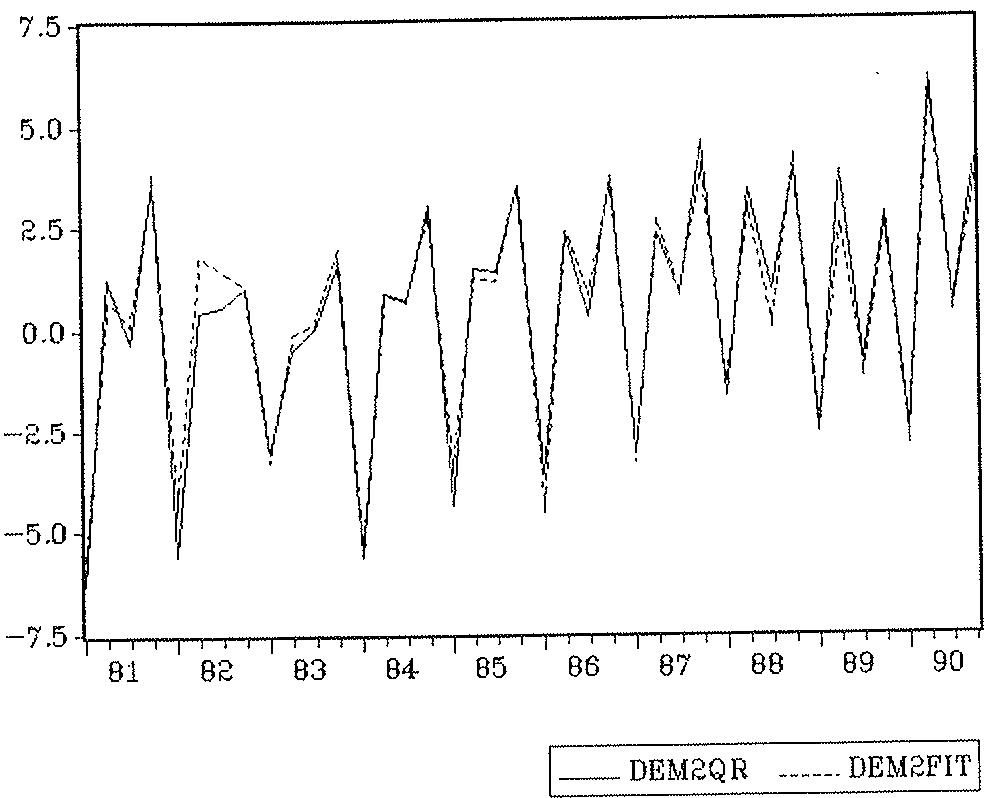
As can be seen from equations (22) to (24), the null hypotheses of no error correction are rejected in all cases at the 1% level, given further support to the cointegration equations (19) to (21) as long-run relationships [see Kremers et al. (1992)]. The signs of the coefficients agree again with our priors, being also statistically significant. Figures 1 to 3 plot the actual and fitted values of the dependent variables in equations (22) to (24), respectively.
TABLE 2: SHORT-RUN RELATIONSHIPS
We have included in equation (22), that is, the equation for the capital account balance, the variable KC (see Appendix 1 for the exact definition), which proxies the effects of capital controls by measuring deviations from covered interest parity. These deviations would signal the presence of unexploited arbitrage profits which can be attributed to the active use of capital controls; see, e. g., Giavazzi and Pagano (1985) or Viñals (1992). Notice that capital controls are not included in the long-run relationship (19) since, as is usually asserted in the literature, even permanent controls would have only temporary effects. Gros (1987) provides a formal assessment of the argument on the long-run ineffectiveness of capital controls, in terms of a model in which economic agents can evade the controls by incurring some costs: the interest differentials created by capital controls would provide an incentive for capital flows, which in turn would work to eliminate those differentials in the long-run.
Notice also that both the money demand and supply equations include seasonal dummies, and a short-run effect is also found for the foreign interest rate and domestic wealth in equation (23), and for the currency-deposits and required-reserves ratios in equation (24).
Together with the adjusted and the standard error of the regression ( ), Table 2 also includes some diagnostic statistics for testing against various alternative hypotheses: residual autocorrelation (DW, Ljung-Box Q and LM), autoregressive conditional heteroscedasticity (ARCH), skewness and excess kurtosis (N), and parameter stability (CHOW) taking as the breaking point the date of the Spanish integration into the EC (the first quarter of 1986) . The tests are distributed as or , where the degrees of freedom are in parentheses. Neither test show any sign of misspecification for equations (22) to (24).
An additional Chow test in equation (24) to assess a possible structural change in the second quarter of 1984, following a change in the Bank of Spain's policy instrument [see note (7)], gave the (non-significant) value CHOW(12,16)=1.90.
Finally, we have tried to address the so-called "Lucas critique". As it is well known, Lucas (1976) questioned the appropriateness of using econometric models for policy simulation experiments, on the grounds that the model's parameters would not be invariant following a change in expectations held by economic agents. Therefore, for an econometric model being able to be used in policy analysis, it is necessary that its parameters show constancy and structural invariance (see, e. g., Ericsson et al., 1991).
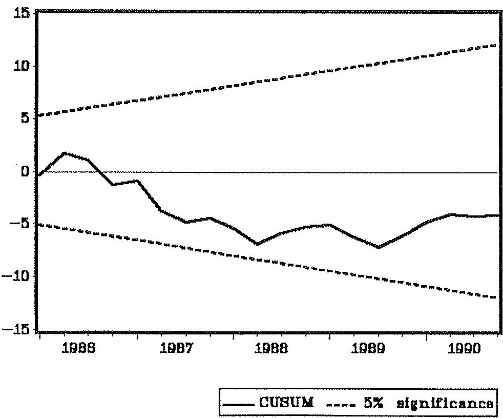
To this end, we have tested for super exogeneity both indirectly via test of constancy and directly via test of structural invariance. In addition to the above standard Chow tests, recursive least squares and the associated sequence of test statistics provide supplementary tools for investigating constancy. Figures 4 to 6 show the CUSUM tests proposed by Brown et al., (1975), together with estimated standard errors. As can be seen, since the test statistics move inside the critical lines, there seems to be no signs of parameter instability .
On the other hand, structural invariance and policy exogeneity was tested by using the procedure suggested by Charemza and Király (1988), which is based on testing recursive residuals of the model as being statistically independent from the examined variables. After applying this test to equations (22) and (24), looking at the exogeneity properties of and KC, as well as H, z, and , respectively, we found
±2
. Plots of the recursive coefficient estimates together with their sequentially estimated standard errors (not reported here, but available from the authors) show that these estimates vary only slightly relative to their ex ante standard errors, giving further support to our hypothesis of parameter constancy.
F-statistics of and . As can be seen, these test statistics are below their critical values and therefore do not suggest the rejection of the invariance hypothesis for those regressors.
Figure 1: Actual and fitted values of in equation (22)
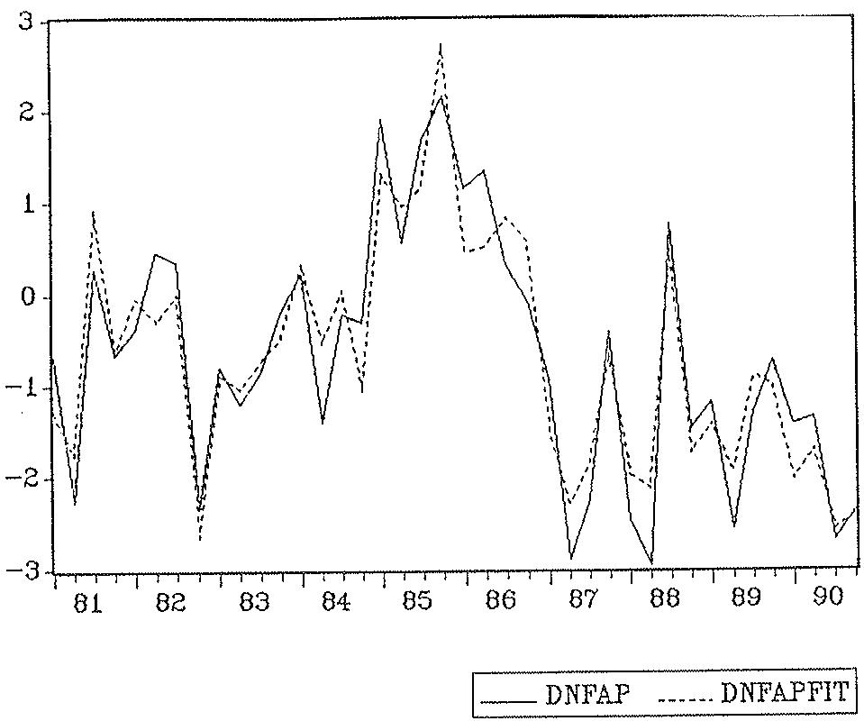
Figure 2: Actual and fitted values of in equation (23)
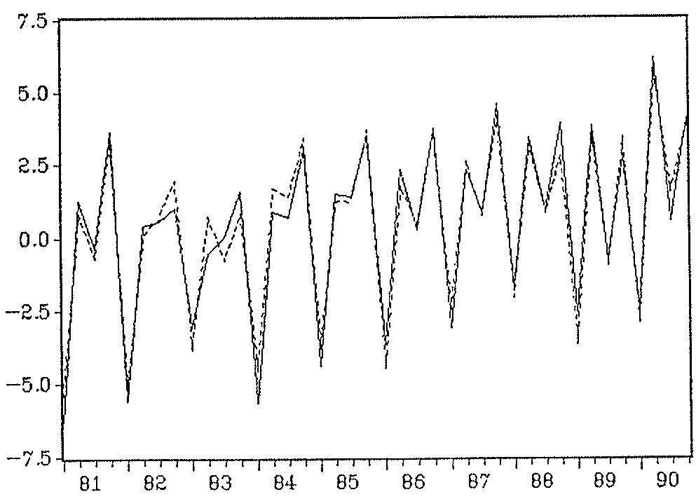
Figure 5: CUSUM test for equation (23) Figure 6: CUSUM test for equation (24)
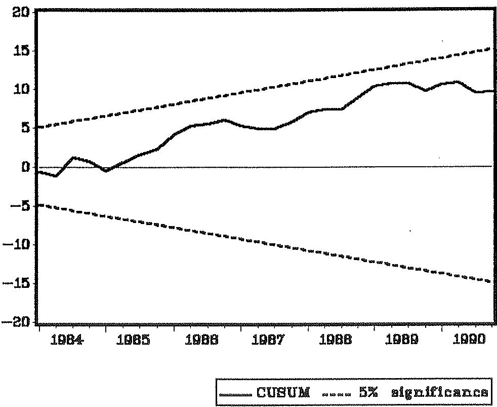
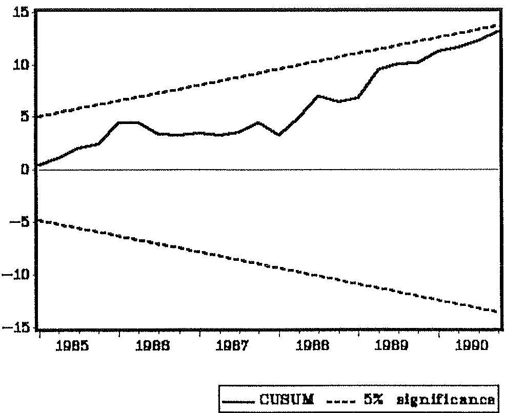
Figure 3: Actual and fitted values of in equation (24) Figure 4: CUSUM test for equation (22)
4.- SIMULATIONS
In this section we discuss the results obtained from simulating changes in some of the model's exogenous variables, on the behaviour of the system given by equations (22) to (24) in Table 2, and allowing the error-correction terms to be continuously updated. The detailed results are presented in Tables and Figures A4.1 to A4.7 in Appendix 4 where, for each of the endogenous variables of the system (i. e., NFAP, M2, and i), we show the change in that variable, computed as the difference between the simulated and the base series.
The following simulations have been performed:
1) A complete elimination of capital controls (i. e., setting KC equal to zero).
2) A transitory 10 per cent increase in the foreign reserves component of the monetary base, distributed among four quarters.
3) A transitory 10 per cent increase in the domestic credit component of the monetary base, distributed among four quarters.
4) A transitory 10 per cent increase in foreign reserves compensated by an equal decrease in domestic credit, distributed among four quarters.
5) A 5 per cent increase in the foreign interest rate during the first quarter, followed by increases of 10, 15 and 20 per cent during the next second, third, and fourth quarters, respectively.
6) A transitory 5 per cent increase in foreign income, distributed among four quarters.
7) A transitory 10 per cent increase in the Pta/US$ forward premium lasting four quarters, proxying a higher expected depreciation of the Peseta.
All simulations have been run from the first to the fourth quarters of 1986, except for the elimination of capital controls. In this case, the simulation runs from the first quarter of 1986 to the end of the sample.
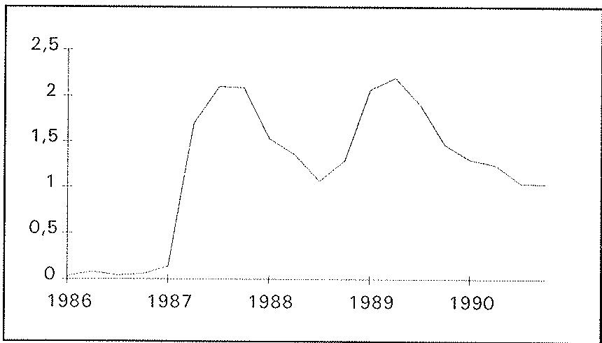
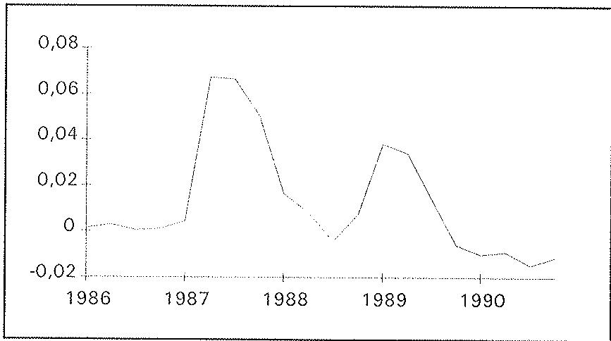
As shown in Table A4.1 and Figure A4.1, the elimination of capital controls would lead to an increase in the net foreign asset position or, in other words, net foreign liabilities would be reduced (i. e., the capital account would worsen). The effect would be specially higher from the second quarter of 1987 and during 1989, that is, the periods where capital controls were more binding [see Viñals (1992)]. This in turn would raise domestic wealth, and hence money demand, the interest rate, and then money supply. However, the increased money supply would reduce the interest rate, which would tend to lower the increase in the net foreign asset position, leading to a subsequent decrease in wealth and money demand. Notice finally that, unlike the other simulations, this is performed in a permanent manner so its effects should be more lasting.
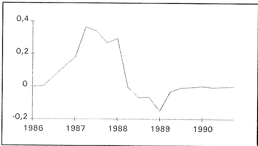
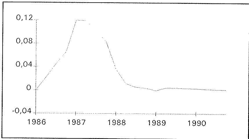
The results from changes in the monetary base are reported in Tables A4.2 to A4.4 and Figures A4.2 to A4.4, and are based in an alternative specification of equations (21) and (24) in which the monetary base is split in its two components of foreign reserves and domestic credit. As can be seen, in all the cases considered, money supply would increase, reducing the interest rate, and the net foreign asset position would increase, both through a higher wealth and a lower domestic interest rate. These effects would be subsequently smoothed by the increase in money demand, which would rise the interest rate. Notice that the effects would be higher when foreign reserves (Table A4.2 and Figure A4.2), instead of domestic credit (Table A4.3 and Figure A4.3), is the variable of which changes are simulated, since its estimated coefficient in the alternative specification for equation (24) is roughly twice that on domestic credit (0.27 versus 0.15). On the other hand, and for the same reason, when the increase in foreign reserves is fully sterilized by the monetary authorities (Table A4.4 and Figure A4.4), the effects on the endogenous variables would have the same signs, though quantitatively much lower.
A transitory increase in the foreign interest rate (Table A4.5 and Figure A4.5) would increase the net foreign asset position, and through a higher wealth and money demand, would also increase the interest rate and money supply. Then, the higher interest rate would slow down the increase in wealth, which would lead to reductions in both the interest rate and money supply.
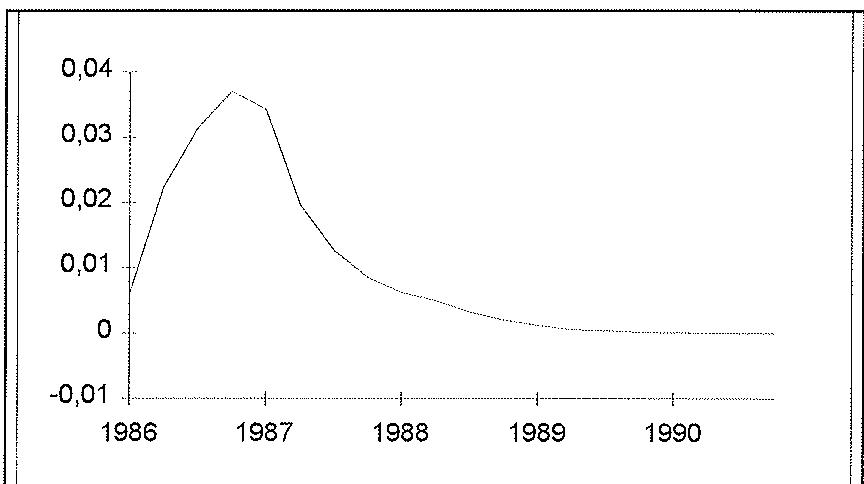
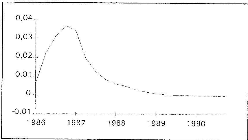
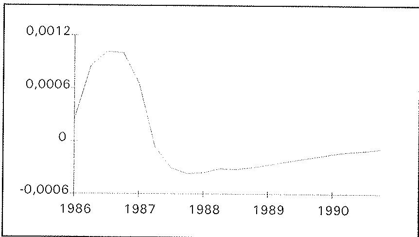
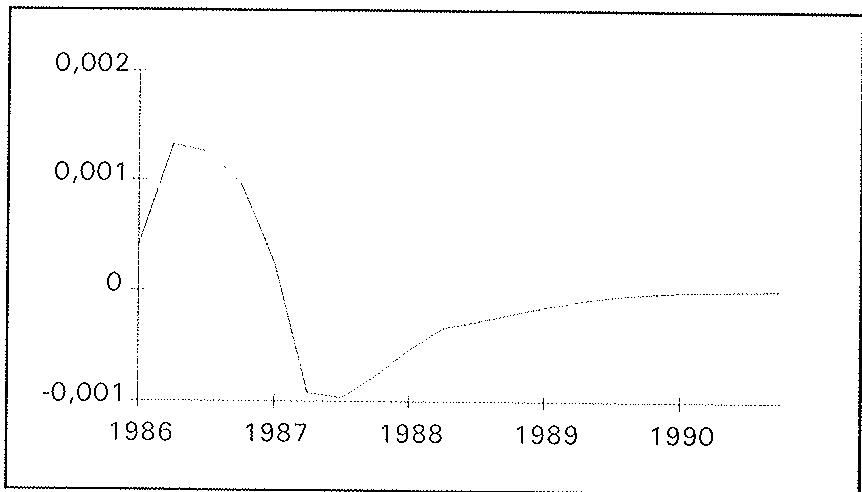
Finally, similar effects would follow from transitory increases in foreign income (Table A4.6 and Figure A4.6) and in the forward premium (Table A4.7 and Figure A4.7), which would be stronger and weaker, respectively, than those derived from a higher foreign interest rate. Once again, the reason should be found in the relative size of the estimated coefficients for those variables in equation (22): 1.68 for foreign income and 0.07 for the forward premium as compared to 0.45 for the foreign interest rate.
FIGURE A4.1: EFFECTS OF AN ELIMINATION OF CAPITAL CONTROLS.
Deviation of NFAP from baseline
Deviation of M2 from baseline
Deviation of i from baseline
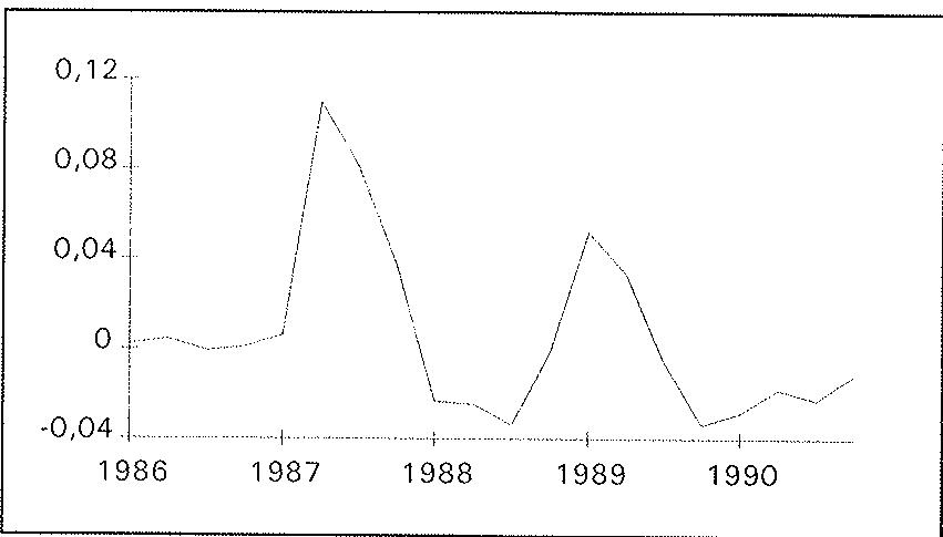
FIGURE A4.2: EFFECTS OF AN INCREASE IN FOREIGN RESERVES.
Deviation of NFAP from baseline.
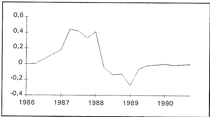
Deviation of M2 from baseline.
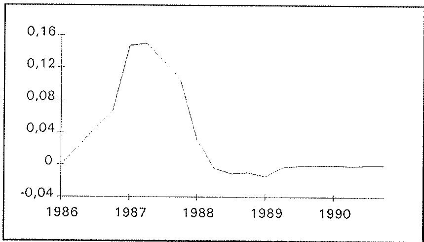
Deviation of i from baseline.
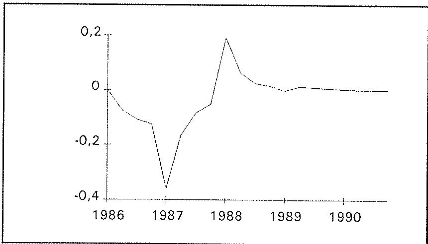
FIGURE A4.3: EFFECTS OF AN INCREASE IN DOMESTIC CREDIT
Deviation of NFAP from baseline
Deviation of M2 from baseline
Deviation of i from baseline
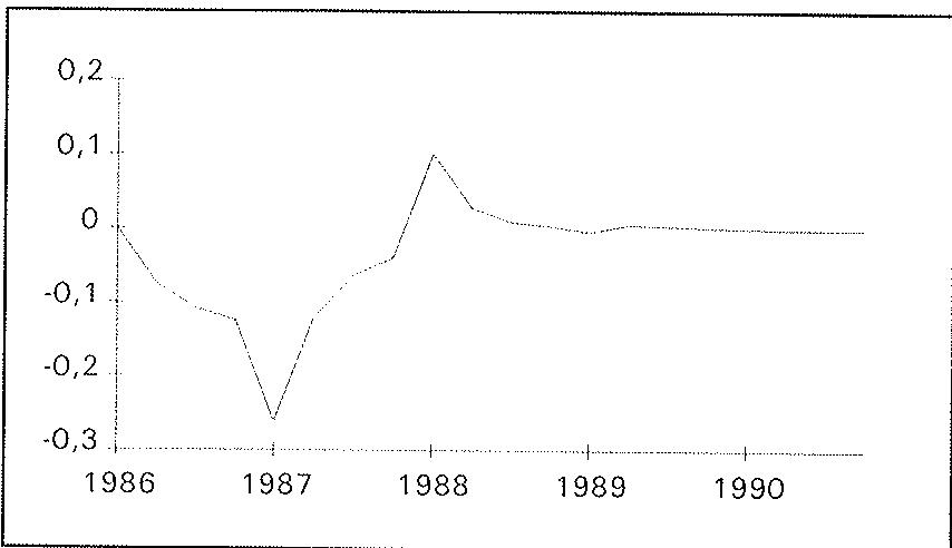
FIGURE A4.4: EFFECTS OF AN INCREASE IN FOREIGN RESERVES, FULLY STERILIZED.
Deviation of NFAP from baseline.
Deviation of M2 from baseline.
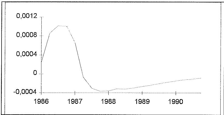
Deviation of i from baseline.
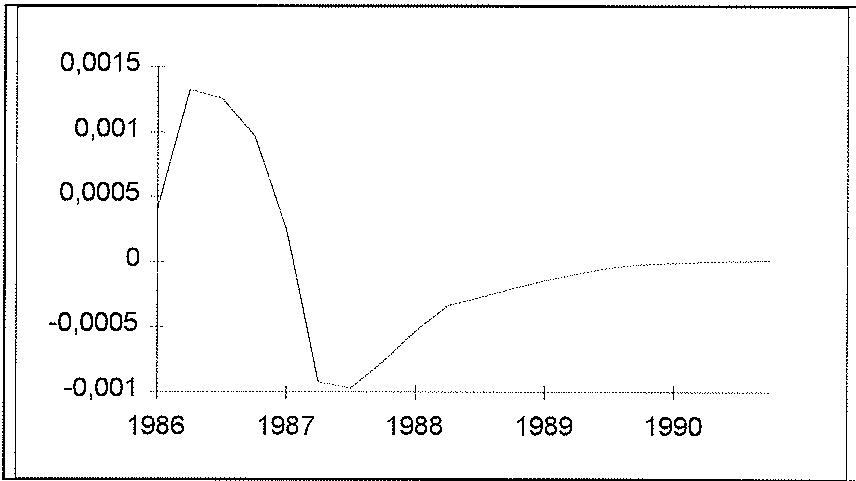
FIGURE A4.5: EFFECTS OF AN INCREASE IN THE FOREIGN INTEREST RATE.
Deviation of NFAP from baseline
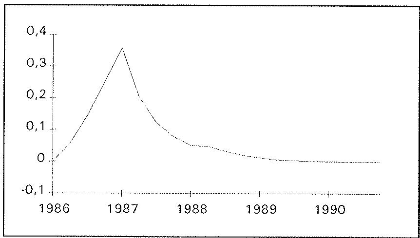
Deviation of M2 from baseline.
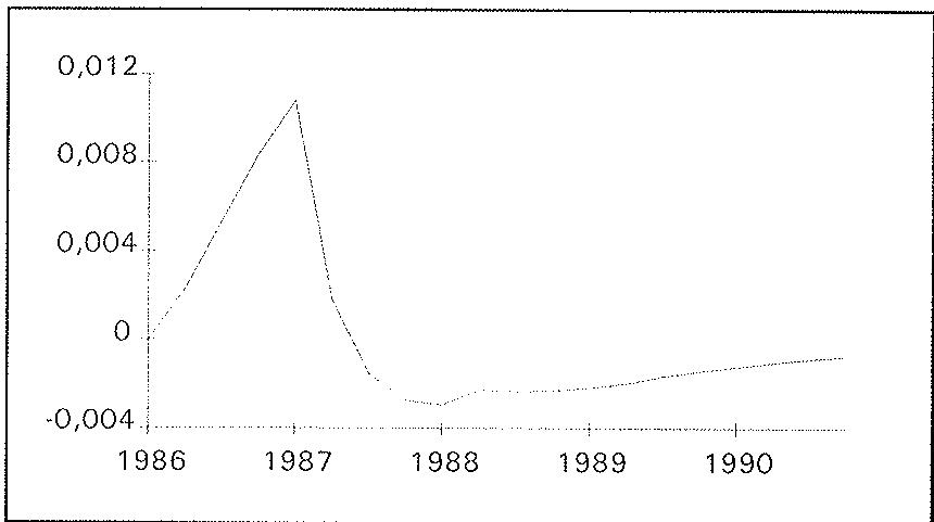
Deviation of i from baseline.
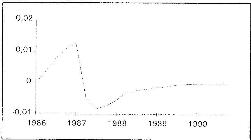
FIGURE A4.6: EFFECTS OF AN INCREASE IN FOREIGN INCOME.
Deviation of NFAP from baseline.
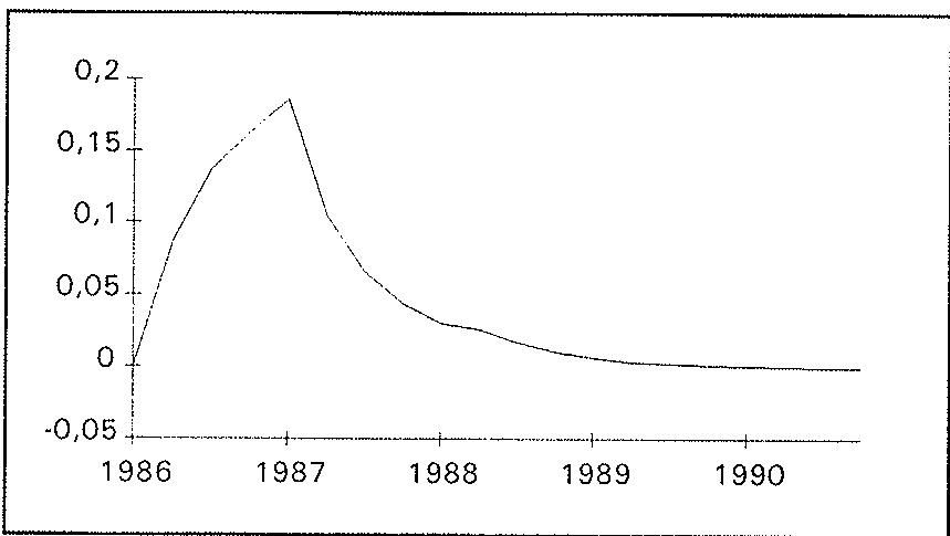
Deviation of M2 from baseline.
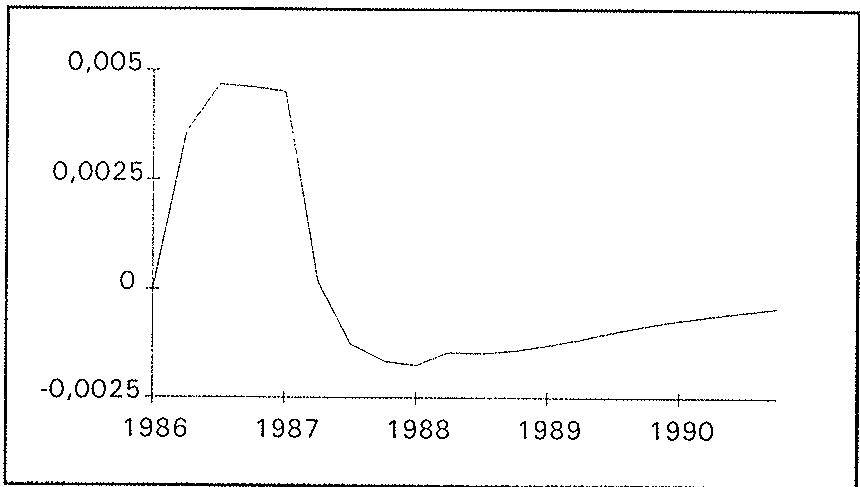
Deviation of i from baseline.
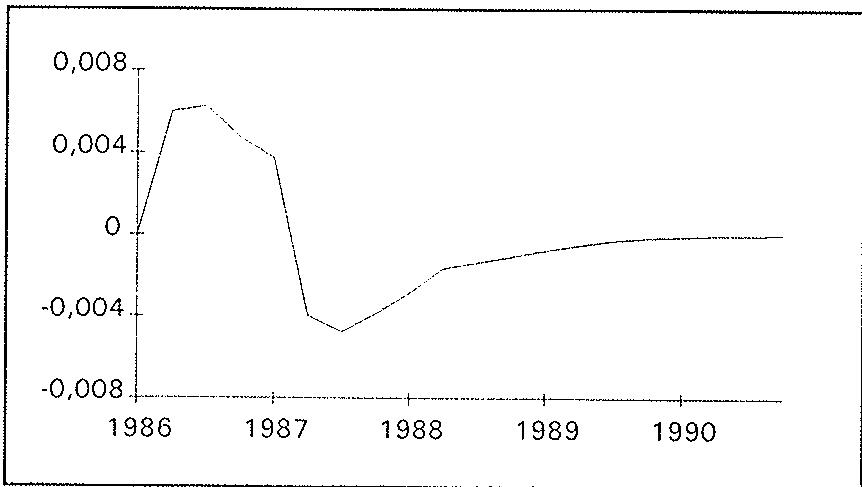
FIGURE A4.7: EFFECTS OF AN INCREASE IN THE FORWARD PREMIUM.
Deviation of NFAP from baseline.
Deviation of M2 from baseline.
Deviation of i from baseline
5. CONCLUSIONS
In this paper we have tried to evaluate the main determinants of capital movements in the Spanish economy by making use of the portfolio-balance approach. A model of three equations was proposed, including equations for the net foreign asset position of the economy together with the demand for and supply of money. The model was estimated with quarterly data for the period 1980.1 through 1990.4, using robust cointegration methods. An interesting feature of the model specification used in the paper is that, given our econometric methodology, it allows us to get estimates of both the net claims on foreigners and their change, which amounts to the capital account balance.
The results of the estimations show a stronger effect from the domestic, as compared to the foreign, interest rate, on the net foreign asset position of the Spanish economy during the above-mentioned period. Other variables showing a significant influence were domestic wealth, and foreign and domestic income levels. On the other hand, capital controls, proxied by deviations in covered interest parity, proved also to play a significant role in the short-run. The model was completed by jointly estimating standard demand for and supply of money equations, and changes in some of the model's exogenous variables were then simulated, showing their effects on the behaviour of the system.
To conclude, notice that the flexibility of the specification proposed along this paper would also allow to estimate alternative models. A natural extension would be the elimination of foreign assets by Walras's law, so that the focus of the analysis would be domestic bonds, together with the money market.
Appendix 1. Definitions of the variables and data sources
\[\mathbf {i} _ {\mathrm{CB}}\]
\[\mathrm{i} _ {\mathbf {M}}\]
\[\mathbf {i} _ {\mathbb {R}}\]
i* = Long-run foreign interest rate, computed as a weighted average, according to their share on Spanish foreign debt, of the yields on long-run government bonds from the US, Switzerland, Germany, Japan, the UK and France
KC = Proxy for the effect of capital controls, measured as deviations from covered interest parity, and computed as the difference between the three-month Spanish interbank and Euro-dollar rates and the Pta-US$ three-month forward premium
M2 = M2 definition of money supply (consisting of currency, and sight and saving deposits) (hundreds of billion Pta), in real terms
NFAP = Net foreign asset position of the Spanish economy, computed as the difference between total foreign assets held by domestic residents (net of official reserves) and total liabilities to foreigners (both in hundreds of billion Pta), in real terms
\[\mathbf {Y}\]
Y* = Imports of the industrialized countries (hundreds of billion US $), in real terms
ε = Pta-US$ three-month forward premium
All the variables in real terms have been deflated by the consumption price index. The Spanish data are taken from the Bank of Spain, except those for the net claims on government, that come from the IMF's International Financial Statistics (line 32an minus line 12a). Most of the Bank of Spain's variables appear in its Boletín Estadístico, except for i and iM, taken from Cuenca (1993); iCB, iR and z, provided by J. L. Escrivá; and Y, provided by P. L'Hotellerie. Regarding the foreign variables, the interest rates and the OECD consumption price index (excluding Turkey) are taken from the OECD's Main Economic Indicators, whereas the nominal imports of the industrialized countries come from the IMF's International Financial Statistics.
Appendix 2. Testing for unit roots
Several statistical tests for unit roots have been developed to test for stationarity in time series. In this paper we have used the non-parametric tests proposed by Phillips and Perron (1988), which are robust to heteroscedasticity, deviations from normality and various forms of serial correlation in the univariate representation of the variables under the unit root null hypothesis.
Phillips and Perron consider three alternative data generating models:
\[X _ {t} = \tilde {\mu} + \tilde {\beta} (t - T / 2) + \tilde {\alpha} X _ {t - 1} + \tilde {\xi} _ {t}\tag{A2.1}\]
\[X _ {t} = \mu^ {*} + \alpha^ {*} X _ {t - 1} + \xi_ {t} ^ {*}\tag{A2.2}\]
and
\[X _ {t} = \hat {\alpha} X _ {t - 1} + \hat {\xi} _ {t}\tag{A2.3}\]
where T is the sample size.
Their approach to testing for unit roots involves estimating the coefficients of these equations by ordinary least squares and constructing the non-parametrically corrected tests statistics , and to test the null hypotheses , and in equation (A2.1), respectively; the statistics and to test the null hypotheses and in equation (A2.2), respectively; and the statistic to test the null hypothesis in equation (A2.3) [see Perron (1988) for a definition of these statistics].
We started by testing for integration of order one on the first differences of the variables, and then went down testing for integration of order zero on the levels of the variables.
Table A2 presents the results from these tests, obtained following the testing sequence proposed by Perron (1988). In addition to the Phillips-Perron tests, we also show those proposed by Bhargava (1986) (denoted R1 and R2) that are valid in small samples and are independent of the nuisance parameters . As can be seen, the null hypothesis of I(2) processes is rejected at the 1% level of significance, whereas the null hypothesis of I(1) is not rejected for all the variables, except for , which would prove to be an I(0) variable.
Note that the critical values for the R1 and R2 tests are only available for a 5% significance level (Bhargava, 1986).
Table A2: Tests for Unit Roots
| $\Delta H$ | $\Delta h$ | $\Delta i$ | $\Delta i_{CB}$ | $\Delta i_M$ | $\Delta i_R$ | $\Delta i^*$ | |
| $Z(\phi_3)$ | $94.39^a$ | $27.61^a$ | $16.01^a$ | $141.03^a$ | $10.88^a$ | $67.12^a$ | $91.63^a$ |
| $z(t_a)$ | $-8.80^a$ | $-4.93^a$ | $-4.30^b$ | $-11.34^a$ | $-3.83^b$ | $-7.61^a$ | $-8.61^a$ |
| R1 | $2.27^b$ | $1.73^b$ | $1.35^b$ | $2.63^b$ | $0.84^b$ | $1.96^b$ | $2.24^b$ |
| R2 | $2.25^b$ | $1.20^b$ | $1.07^b$ | $2.27^b$ | $1.20^b$ | $1.96^b$ | $2.23^b$ |
| H | h | i | $i_{CB}$ | $i_M$ | $i_R$ | $i^*$ | |
| $Z(\phi_3)$ | 1.80 | 5.36 | 1.45 | 5.69 | 6.60 | 2.73 | 2.00 |
| $z(t_a)$ | -1.69 | -3.12 | -1.66 | -3.07 | 1.93 | -0.73 | -1.85 |
| $Z(\phi_2)$ | 1.30 | $6.89^b$ | 0.98 | 3.80 | $5.75^b$ | 1.82 | 1.36 |
| $z(t_a')$ | 1.06 | 0.81 | 1.05 | 2.34 | -1.37 | 1.32 | 1.58 |
| $Z(\phi_1)$ | 1.19 | 3.62 | 1.21 | 4.79 | $6.63^b$ | 1.47 | 1.63 |
| $z(t_a)$ | 0.02 | 2.45 | -0.31 | -0.34 | 1.97 | -0.77 | -0.03 |
| R1 | 0.14 | 0.05 | 0.17 | $0.84^b$ | 0.07 | 0.18 | 0.20 |
| R2 | 0.25 | 0.44 | 0.19 | 0.73 | 0.07 | 0.18 | 0.18 |
| $\Delta M2$ | $\Delta NFAP$ | $\Delta W$ | $\Delta Y$ | $\Delta Y^{*}$ | $\Delta z$ | $\Delta \varepsilon$ | |
| $Z(\phi_3)$ | $3015.1^a$ | $10.55^a$ | $188.50^a$ | $20.62^a$ | $363.42^a$ | $42.67.^a$ | $181.90^a$ |
| $z(t_{\tilde{\alpha}})$ | $-49.53^a$ | $-3.50^b$ | $-11.41^a$ | $-4.48^a$ | $-16.22^a$ | $-6.26^a$ | $-12.54^a$ |
| R1 | $2.95^b$ | $1.03^b$ | $2.36^b$ | $0.97^b$ | $2.31^b$ | $1.82^b$ | $2.56^b$ |
| R2 | $3.09^b$ | $1.08^b$ | $2.25^b$ | $1.28^b$ | $2.44^b$ | $1.78^b$ | $2.10^b$ |
| M2 | NFAP | W | Y | Y* | z | ε | |
| $Z(\phi_3)$ | 5.49 | 1.53 | 3.12 | $6.96^b$ | $8.05^b$ | 1.01 | $10.69^a$ |
| $z(t_{\tilde{\alpha}})$ | 1.66 | -0.52 | -2.32 | 0.13 | -1.85 | -0.59 | $-3.90^b$ |
| $Z(\phi_2)$ | 3.86 | 2.65 | 3.61 | $10.56^a$ | 5.44 | 0.67 | $7.20^a$ |
| $z(t_{\tilde{\alpha}}')$ | 0.27 | 0.60 | 0.27 | -1.98 | 1.65 | 0.95 | 2.71 |
| $Z(\phi_1)$ | 1.07 | 2.72 | 1.92 | $13.14^a$ | 0.15 | 0.97 | $10.59^a$ |
| $z(t_{\tilde{\alpha}})$ | 1.18 | 2.22 | 1.89 | 4.15 | 0.53 | -0.69 | $-2.20^b$ |
| R1 | 0.17 | 0.03 | 0.03 | 0.01 | 0.13 | 0.13 | $0.89^b$ |
| R2 | 0.15 | 0.07 | 0.14 | 0.03 | 0.17 | 0.12 | $0.81^b$ |
Note: "a" and "b" denote significance at the 1% and 5% levels, respectively.
Appendix 3. Testing for seasonal unit roots
Due to the fact that the time series used in the paper are quarterly, we have also tested for the presence of unit roots at seasonal frequencies by means of the test proposed by Hylleberg et al. (1990).
These authors present the following two-step procedure test:
1) Compute
\[\mathrm{X} _ {1 1} = (1 + \mathrm{L}) (1 + \mathrm{L} ^ {2}) \mathrm{X} _ {1} = (1 + \mathrm{L} + \mathrm{L} ^ {2} + \mathrm{L} ^ {3}) \mathrm{X} _ {1},\]
\[\mathrm{X} _ {2 \mathrm{t}} = - (1 - \mathrm{L}) (1 + \mathrm{L} ^ {2}) \mathrm{X} _ {\mathrm{t}} = - (1 - \mathrm{L} + \mathrm{L} ^ {2} - \mathrm{L} ^ {3}) \mathrm{X} _ {\mathrm{t}},\]
\[\mathrm{X} _ {3 1} = - (1 - \mathrm{L} ^ {2}) \mathrm{X} _ {1},\]
and
\[\mathrm{X} _ {4 1} = (1 - \mathrm{L} ^ {4}) \mathrm{X} _ {1}.\]
2) Run the auxiliary regression
\[\mathrm{X} _ {4 \mathrm{t}} = \pi_ {1} \mathrm{X} _ {1 \mathrm{t} - 1} + \pi_ {2} \mathrm{X} _ {2 \mathrm{t} - 1} + \pi_ {3} \mathrm{X} _ {3 \mathrm{t} - 2} + \pi_ {4} \mathrm{X} _ {3 \mathrm{t} - 1} + \eta_ {\mathrm{t}}\]
and compute the values of the t-ratios on and , and the F-test on .
This regression may also be extended by including deterministic components such as a constant, a trend, and seasonal dummy variables.
There will be no seasonal unit roots if and either or are different from zero, which therefore requires the rejection of both a test on ( : unit root at the frequency 1/2) and a joint test for and ( : unit root at the frequencies 1/4 and 3/4). If the t-test on is not significant, then the series has a unit root at the zero frequency.
The critical values are given in Table 1 of Hylleberg et al. (1990, pp. 226-227).
Table A3 presents the results of this test for our data set. As can be seen, the t-test on indicates as before a unit root at the zero frequency for all the series (except for ), while the t-test on and the F-test on do not suggest any non-stationarity at the seasonal frequencies.
Table A3: Tests for Seasonal Unit Roots
| Variable | Auxiliary Regression | t: $\pi_1$ | t: $\pi_2$ | t: $\pi_3$ | t: $\pi_4$ | F: $\pi_3 \cap \pi_4$ |
| H | -- | 0.05 | -3.77a | -4.19a | -3.47a | 21.26a |
| C | -1.32 | -3.76a | -4.30a | -3.32a | 21.13a | |
| C, SD | -1.36 | -4.14a | -4.09b | -3.14a | 18.76a | |
| C, T | -1.73 | -3.95a | -4.53a | -3.23a | 22.29a | |
| C, T, SD | -1.68 | -4.31a | -4.31b | -3.03a | 19.80a | |
| h | -- | 3.18 | -3.40a | -1.62 | -4.51a | 15.27a |
| C | -0.08 | -3.36a | -1.60 | -4.40a | 12.82a | |
| C, SD | -0.26 | -4.55a | -1.14 | -3.76a | 7.33b | |
| C, T | -2.30 | -3.52a | -2.20b | -3.93a | 14.94a | |
| C, T, SD | -2.54 | -4.86a | -1.79 | -3.29a | 9.12b | |
| i | -- | 0.36 | -4.78a | -1.52 | -5.26a | 16.81a |
| C | -1.99 | -4.77a | -1.84 | -4.97a | 16.32a | |
| C, SD | -1.93 | -4.64a | -1.76 | -4.80a | 15.13a | |
| C, T | -1.94 | -4.67a | -1.81 | -4.92a | 15.95a | |
| C, T, SD | -1.88 | -4.55a | -1.73 | -4.75a | 14.76a | |
| $i_{CB}$ | -- | 0.24 | -2.62b | -4.06a | -3.54a | 22.85a |
| C | -2.79 | -2.85a | -4.91a | -3.18a | 27.60a | |
| C, T | -2.76 | -2.84 | -4.77a | -3.10a | 26.77a | |
| C, T | -3.30 | -2.95a | -5.10a | -3.13a | 28.76a | |
| C, T, SD | -3.22 | -2.94 | -4.93a | -3.02a | 27.26a | |
| Variable | Auxiliary Regression | t: π1 | t: π2 | t: π3 | t: π4 | F: π3 ∩ π4 |
| iM | -- | 1.29 | -5.09 | -2.35c | -6.50a | 47.74a |
| C | 3.33 | -4.11 | -2.62b | -4.33 | 23.99a | |
| C, T | 3.59 | -3.84a | -2.67 | -4.21 | 24.39a | |
| C, T | 2.46 | -4.09a | -2.73b | -4.34a | 23.95a | |
| C, T, SD | 2.71 | -3.82a | -2.77 | -4.21a | 24.24a | |
| iR | -- | -0.76 | -3.64a | -3.71a | -3.64a | 27.13a |
| C | -2.00 | -3.51a | -3.85a | -3.68a | 27.30a | |
| C, T | -1.93 | -3.33a | -3.66b | -3.69a | 26.03a | |
| C, T | -1.03 | -3.39a | -3.57a | -3.36a | 21.04a | |
| C, T, SD | -1.01 | -3.22b | -3.38 | -3.39a | 19.95a | |
| i* | -- | 0.02 | -4.66a | -5.34a | -2.70a | 24.60a |
| C | -2.09 | -4.77a | -5.69a | -2.48a | 26.22a | |
| C, T | -2.06 | -5.21a | -5.58a | -2.33b | 14.42a | |
| C, T | -2.33 | -4.73a | -5.66a | -2.34b | 25.24a | |
| C, T, SD | -2.27 | -5.14a | -5.55a | -2.20b | 23.55a | |
| M2 | -- | 1.27 | -1.79c | -3.92a | -3.86a | 21.54a |
| C | 1.57 | -1.73c | -3.73a | -3.60a | 18.30a | |
| C, T | 0.16 | -4.15a | -4.10b | -4.40a | 32.54a | |
| C, T | 2.73 | -1.22 | -2.55b | -2.13b | 6.16a | |
| C, T, SD | 1.12 | -3.52c | -3.32c | -3.87a | 19.42a |
Table A3 (Cont.)
| Variable | Auxiliary Regression | t: $\pi_1$ | t: $\pi_2$ | t: $\pi_3$ | t: $\pi_4$ | F: $\pi_3 \cap \pi_4$ |
| NFAP | -- | 1.20 | -4.83a | -3.11a | -5.71a | 33.38a |
| C | 0.53 | -4.47a | -3.06a | -5.65a | 32.67a | |
| C, T | 0.51 | -4.78a | -2.64a | -5.73a | 30.59a | |
| C, T | -1.70 | -4.82a | -3.77a | -5.11a | 35.48a | |
| C, T, SD | -1.70 | -4.88a | -3.38a | -5.16a | 33.22a | |
| W | -- | 2.03b | -3.07a | -5.12a | -4.13a | 37.57a |
| C | -0.38 | -3.03a | -5.16a | -4.02a | 37.33a | |
| C, T | -0.78 | -3.47b | -4.96a | -4.00a | 39.21a | |
| C, T | -1.67 | -3.08a | -5.26a | -3.86a | 36.67a | |
| C, T, SD | -1.60 | -3.51b | -5.07a | -3.77a | 38.28a | |
| Y | -- | 2.26 | -7.32a | -0.72 | -3.96a | 8.31a |
| C | 2.86 | -6.00a | -0.52 | -4.19a | 9.08a | |
| C, T | 2.78 | -5.78a | -0.47 | -4.12a | 8.75a | |
| C, T | -0.12 | -0.82 | -0.65 | -4.10a | 9.23a | |
| C, T, SD | -0.10 | -5.59a | -0.60 | -4.13a | 8.92a | |
| Y* | -- | 1.38 | -2.41b | -3.96a | -4.55a | 32.93a |
| C | -0.10 | -2.39b | -3.91a | -4.42a | 32.35a | |
| C, T | -0.66 | -2.81c | -3.34c | -5.73a | 48.04a | |
| C, T | -0.53 | -2.38b | -3.91a | -4.36a | 31.74a | |
| C, T, SD | -1.08 | -2.80c | -3.46c | -5.54a | 47.68a | |
| z | -- | -0.65 | $-3.47^a$ | $-3.15^a$ | $-3.49^a$ | $23.17^a$ |
| C | -1.43 | $-3.43^a$ | $-3.23^a$ | $-3.45^a$ | $23.59^a$ | |
| C, T | -1.39 | $-3.30^b$ | -3.11 | $-3.22^a$ | $22.00^a$ | |
| C, T | -0.62 | $-3.39^a$ | $-3.13^a$ | $-3.55^a$ | $19.96^a$ | |
| C, T, SD | -0.60 | $-3.26^b$ | $-3.02^a$ | $-3.12^a$ | $18.58^a$ | |
| ε | -- | -1.55 | $-5.05^a$ | $-5.15^a$ | $-2.50^b$ | $20.97^a$ |
| C | $-3.65^b$ | $-5.52^a$ | $-5.54^a$ | $-2.19^b$ | $22.02^a$ | |
| C, T | $-3.51^b$ | $-5.56^a$ | $-5.98^a$ | $-2.23^b$ | $26.22^a$ | |
| C, T | $-3.56^b$ | $-5.48^a$ | $-5.48^a$ | $-2.17^b$ | $21.41^a$ | |
| C, T, SD | $-3.48^c$ | $-5.52^a$ | $5.93^a$ | $-2.22^b$ | $30.91^a$ |
(ii) "a", "b" and "c" denote significance at the 1%, 5% and 10% levels, respectively. Notes: (i) "C", "SD", and "T" denote constant, seasonal dummies and trend, respectively.
Appendix 4. Simulation results
| Table A4.1:Effects of an Elimination of Capital Controls* | |||
| NFAP | M2 | i | |
| 1986.1 | 0.0314 | 0.0013 | 0.0022 |
| 1986.2 | 0.0825 | 0.0031 | 0.0046 |
| 1986.3 | 0.0394 | 0.0005 | -0.0008 |
| 1986.4 | 0.0569 | 0.0012 | 0.0007 |
| 1987.1 | 0.1397 | 0.0044 | 0.0060 |
| 1987.2 | 1.6949 | 0.0674 | 0.1100 |
| 1987.3 | 2.1024 | 0.0066 | 0.0806 |
| 1987.4 | 2.0924 | 0.0503 | 0.0366 |
| 1988.1 | 1.5294 | 0.0164 | -0.0233 |
| 1988.2 | 1.3645 | 0.0080 | -0.0246 |
| 1988.3 | 1.0693 | -0.0042 | -0.0337 |
| 1988.4 | 1.2913 | 0.0075 | -0.0019 |
| 1989.1 | 2.0683 | 0.0383 | 0.0520 |
| 1989.2 | 2.1962 | 0.0341 | 0.0332 |
| 1989.3 | 1.9025 | 0.0143 | -0.0053 |
| 1989.4 | 1.4649 | -0.0059 | -0.0339 |
| 1990.1 | 1.3000 | -0.0099 | -0.0286 |
| 1990.2 | 1.2434 | -0.0090 | -0.0181 |
| 1990.3 | 1.0442 | -0.0146 | -0.0225 |
| 1990.4 | 1.0384 | -0.0111 | -0.0111 |
| * Deviation from baseline | |||
| Table A4.2:Effects of an Increase in Foreign Reserves | |||
| NFAP | M2 | i | |
| 1986.1 | 0.0000 | 0.0000 | 0.0000 |
| 1986.2 | 0.0027 | 0.0215 | -0.0753 |
| 1986.3 | 0.0618 | 0.0451 | -0.1086 |
| 1986.4 | 0.1231 | 0.0657 | -0.1242 |
| 1987.1 | 0.1806 | 0.1475 | -0.3602 |
| 1987.2 | 0.4421 | 0.1496 | -0.1637 |
| 1987.3 | 0.4194 | 0.1284 | -0.0838 |
| 1987.4 | 0.3317 | 0.1052 | -0.0517 |
| 1988.1 | 0.4131 | 0.0304 | 0.1927 |
| 1988.2 | -0.0445 | -0.0046 | 0.0632 |
| 1988.3 | -0.1349 | -0.0109 | 0.0254 |
| 1988.4 | -0.1247 | -0.0098 | 0.0137 |
| 1989.1 | -0.2705 | -0.0148 | -0.0024 |
| 1989.2 | -0.0630 | -0.0033 | 0.0132 |
| 1989.3 | -0.0192 | -0.0015 | 0.0095 |
| 1989.4 | -0.0098 | -0.0014 | 0.0054 |
| 1990.1 | 0.0022 | -0.0009 | 0.0035 |
| 1990.2 | -0.0131 | -0.0015 | 0.0007 |
| 1990.3 | -0.0058 | -0.0010 | 0.0009 |
| 1990.4 | -0.0010 | -0.0007 | 0.0008 |
| * Deviation from baseline | |||
| Table A4.3:Effects of an Increase in Domestic Credit | |||
| NFAP | M2 | i | |
| 1986.1 | 0.0000 | 0.0000 | 0.0000 |
| 1986.2 | 0.0027 | 0.0215 | -0.0753 |
| 1986.3 | 0.0618 | 0.0451 | -0.1086 |
| 1986.4 | 0.1231 | 0.0657 | -0.1242 |
| 1987.1 | 0.1771 | 0.1194 | -0.2616 |
| 1987.2 | 0.3648 | 0.1187 | -0.1201 |
| 1987.3 | 0.3391 | 0.1014 | -0.0634 |
| 1987.4 | 0.2671 | 0.0829 | -0.0400 |
| 1988.1 | 0.2933 | 0.0360 | 0.1013 |
| 1988.2 | -0.0058 | 0.0115 | 0.0285 |
| 1988.3 | -0.0673 | 0.0053 | 0.0094 |
| 1988.4 | -0.0650 | 0.0039 | 0.0045 |
| 1989.1 | -0.1492 | -0.0006 | -0.0035 |
| 1989.2 | -0.0317 | 0.0047 | 0.0060 |
| 1989.3 | -0.0089 | 0.0044 | 0.0043 |
| 1989.4 | -0.0047 | 0.0036 | 0.0022 |
| 1990.1 | 0.0018 | 0.0031 | 0.0013 |
| 1990.2 | -0.0070 | 0.0021 | -0.0001 |
| 1990.3 | -0.0027 | 0.0019 | 0.0001 |
| 1990.4 | -0.0001 | 0.0016 | 0.0002 |
| * Deviation from baseline | |||
| Table A4.4: Effects of an Increase in Foreign Reserves, Fully Sterilized | |||
| NFAP | M2 | i | |
| 1986.1 | 0.0000 | 0.0000 | 0.0000 |
| 1986.2 | 0.0000 | 0.0000 | 0.0000 |
| 1986.3 | 0.0000 | 0.0000 | 0.0000 |
| 1986.4 | 0.0000 | 0.0000 | 0.0000 |
| 1987.1 | 0.0035 | 0.0281 | -0.0986 |
| 1987.2 | 0.0773 | 0.0309 | -0.0436 |
| 1987.3 | 0.0803 | 0.0270 | -0.0204 |
| 1987.4 | 0.0646 | 0.0223 | -0.0118 |
| 1988.1 | 0.1198 | -0.0056 | 0.0914 |
| 1988.2 | -0.0387 | -0.0161 | 0.0348 |
| 1988.3 | -0.0675 | -0.0161 | 0.0150 |
| 1988.4 | -0.0597 | -0.0137 | 0.0091 |
| 1989.1 | 0.1214 | -0.0142 | 0.0011 |
| 1989.2 | -0.0313 | -0.0079 | 0.0071 |
| 1989.3 | -0.0102 | -0.0060 | 0.0053 |
| 1989.4 | -0.0052 | 0.0049 | 0.0032 |
| 1990.1 | 0.0004 | 0.0040 | 0.0022 |
| 1990.2 | -0.0062 | -0.0036 | 0.0008 |
| 1990.3 | -0.0031 | -0.0023 | 0.0008 |
| 1990.4 | -0.001 | -0.0023 | 0.0007 |
| * Deviation from baseline | |||
| Table A4.5:Effects of an Increase in the Foreign Interest Rate* | |||
| NFAP | M2 | i | |
| 1986.1 | 0.0000 | 0.0000 | 0.0000 |
| 1986.2 | 0.0060 | 0.0023 | 0.0039 |
| 1986.3 | 0.1447 | 0.0053 | 0.0080 |
| 1986.4 | 0.2497 | 0.0083 | 0.0110 |
| 1987.1 | 0.3594 | 0.0108 | 0.0127 |
| 1987.2 | 0.2038 | 0.0018 | -0.0049 |
| 1987.3 | 0.1230 | -0.0015 | -0.0082 |
| 1987.4 | 0.0776 | -0.0027 | -0.0073 |
| 1988.1 | 0.0570 | -0.0030 | -0.0055 |
| 1988.2 | 0.0477 | -0.0023 | -0.0028 |
| 1988.3 | 0.0332 | -0.0023 | -0.0023 |
| 1988.4 | 0.0209 | -0.0023 | -0.0019 |
| 1989.1 | 0.0125 | -0.0022 | -0.0014 |
| 19892. | 0.0065 | -0.0020 | -0.0010 |
| 1989.3 | 0.0041 | -0.0017 | -0.0005 |
| 1989.4 | 0.0025 | -0.0014 | -0.0003 |
| 1990.1 | 0.0013 | -0.0012 | -0.0001 |
| 1990.2 | 0.0005 | -0.0010 | 0.0000 |
| 1990.3 | 0.0000 | -0.0009 | 0.0000 |
| 1990.4 | 0.0000 | -0.0007 | 0.0000 |
| * Deviation from baseline | |||
| Table A4.6:Effects of an Increase in Foreign Income | |||
| NFAP | M2 | i | |
| 1986.1 | 0.0000 | 0.0000 | 0.0000 |
| 1986.2 | 0.0872 | 0.0036 | 0.0060 |
| 1986.3 | 0.1364 | 0.0047 | 0.0063 |
| 1986.4 | 0.1628 | 0.0046 | 0.0048 |
| 1987.1 | 0.1858 | 0.0045 | 0.0037 |
| 1987.2 | 0.1044 | 0.0002 | -0.0040 |
| 1987.3 | 0.0655 | -0.0013 | -0.0048 |
| 1987.4 | 0.0440 | -0.0017 | -0.0039 |
| 1988.1 | 0.0300 | -0.0017 | -0.0029 |
| 1988.2 | 0.0259 | -0.0015 | -0.0016 |
| 1988.3 | 0.0173 | -0.0015 | -0.0013 |
| 1988.4 | 0.0107 | -0.0014 | -0.0011 |
| 1989.1 | 0.0064 | -0.0013 | -0.0007 |
| 1989.2 | 0.0034 | -0.0012 | -0.0005 |
| 1989.3 | 0.0022 | -0.0010 | -0.0003 |
| 1989.4 | 0.0012 | -0.0008 | -0.0001 |
| 1990.1 | 0.0006 | -0.0007 | -0.0001 |
| 1990.2 | 0.0002 | -0.0006 | -0.0001 |
| 1990.3 | 0.0000 | -0.0005 | 0.0000 |
| 1990.4 | 0.0000 | -0.0004 | 0.0000 |
| * Deviation from baseline | |||
| Table A4.7: effects of an Increase in the Forward Premium* | |||
| NFAP | M2 | i | |
| 1986.1 | 0.0006 | 0.0002 | 0.0004 |
| 1986.2 | 0.0223 | 0.0009 | 0.0013 |
| 1986.3 | 0.0315 | 0.0010 | 0.0013 |
| 1986.4 | 0.0370 | 0.0010 | 0.0010 |
| 1987.1 | 0.0343 | 0.0007 | 0.0002 |
| 1987.2 | 0.0197 | -0.0001 | -0.0009 |
| 1987.3 | 0.0126 | -0.0003 | -0.0010 |
| 1987.4 | 0.0085 | -0.0004 | -0.0008 |
| 1988.1 | 0.0062 | -0.0004 | -0.0005 |
| 1988.2 | 0.005 | -0.0003 | -0.0003 |
| 1988.3 | 0.0033 | -0.0003 | -0.0003 |
| 1988.4 | 0.0020 | -0.0003 | -0.0002 |
| 1989.1 | 0.0012 | -0.0003 | -0.0001 |
| 1989.2 | 0.0006 | -0.0002 | -0.0001 |
| 1989.3 | 0.0004 | -0.0002 | -0.0001 |
| 1989.4 | 0.0002 | -0.0002 | 0.0000 |
| 1990.1 | 0.0001 | -0.0001 | 0.0000 |
| 1990.2 | 0.0001 | -0.0001 | 0.0000 |
| 1990.3 | 0.0000 | -0.0001 | 0.0000 |
| 1990.4 | 0.0000 | -0.0001 | 0.0000 |
| * Deviation from baseline | |||
References
Argy, V. and Kouri, P. J. K. (1974): "Sterilization policies and the volatility in international reserves", in R. Z. Aliber (ed.): National monetary policies and the international financial system, The University of Chicago Press, Chicago, 209-230.
Baba, Y., Hendry, D. F. and Starr, R. M. (1992): "The demand for M1 in the USA, 1960-1988", Review of Economic Studies 59, 25-61.
Bajo-Rubio, O. and Sosvilla-Rivero, S. (1994): "An econometric analysis of foreign direct investment in Spain, 1964-89", forthcoming in Southern Economic Journal.
Baulant, C. and Boutillier, M. (1992): "Foreign position in French francs. An econometric study with stock data over the EMS period", Economic Modelling 9, 290-300.
Bhargava, A. (1986): "On the theory of testing for unit roots in observed time series", Review of Economic Studies 53, 369-384.
Branson, W. H. (1968): Financial capital flows in the U.S. balance of payments, North-Holland, Amsterdam.
Branson, W. H. and Henderson, D. W. (1985): "The specification and influence of asset markets", in R. W. Jones and P. B. Kenen (eds.): Handbook of International Economics (vol. II), North-Holland, Amsterdam, 749-805.
Brown, R. L., Durbin, J. and Evans, J. M. (1975): "Techniques for testing the constancy of regression relationships over time", Journal of the Royal Statistical Society, Series B, 37, 149-163.
Campbell, J. Y. and Perron, P. (1992): "Pitfalls and opportunities: what macroeconomists should know about unit roots", NBER Macroeconomics Annual 7, 141-201.
- Carrascosa, A. and Sastre, L. (1992): "Evolución y determinantes de la inversión extranjera en inmuebles en España", Moneda y Crédito 194, 245-269.
- Charemza, W. and Király, J. (1988): "A simple test for structural invariance and policy exogeneity", Discussion Paper No. 95, Department of Economics, University of Leicester, Leicester.
- Claassen, E. M. and Wyplosz, C. (1982): "Capital controls: some principles and the French experience", Annales de l'INSEE 47-48, 237-267.
- Cuenca, J. A. (1993): "La construcción de variables financieras para el estudio del sector monetario de la economía española", Documento EC/1993/16, Servicio de Estudios, Banco de España, Madrid.
- Dolado, J. J. (1988): "Innovación financiera, inflación y estabilidad de la demanda de ALP en España", Boletín Económico, Banco de España, april, 19-35.
- Dolado, J. J. (1989): "Cointegración: una panorámica", Documento de Trabajo 8902, Banco de España, Madrid.
- Dolado, J. J., Jenkinson, T. and Sosvilla-Rivero, S. (1990): "Cointegration and unit roots", Journal of Economic Surveys 4, 249-273.
- Dornbusch, R. (1983): "Exchange rate risk and the macroeconomics of exchange rate determination", in R. Hawkins, R. Levich and C. G. Wihlborg (eds.): The internationalization of financial markets and national economic policy (vol. 3), JAI Press, Greenwich, CT, 3-27.
- Engle, R. F. and Granger, C. W. J. (1987): "Cointegration and error correction: representation, estimation, and testing", Econometrica 55, 251-276.
- Engle, R. F. and Yoo, B. S. (1987): "Forecasting and testing in cointegrated system", Journal of Econometrics 35, 143-159.
- Ericsson, N. E., Campos, J. and Tran, H.-A. (1991): "PC-GIVE and David Hendry's econometric methodology", International Finance Discussion Paper No. 406, Board of Governors of the Federal Reserve System, Washington, D.C.
- Escrivá, J. L. and Santos, R. (1991): "Un estudio del cambio de régimen en la variable instrumental del control monetario en España", Documento de Trabajo 9111, Banco de España, Madrid.
- Giavazzi, F. and Pagano, M. (1985): "Capital controls and the European Monetary System", in Capital controls and foreign exchange legislation, Occasional Paper, Euromobiliare, Milano, 19-38.
- Gros, D. (1987): "The effectiveness of capital controls: implications for monetary autonomy in the presence of incomplete market separation", International Monetary Fund Staff Papers 34, 621-642.
- Haug, A. A. (1992): "Critical values for the -Phillips-Ouliaris test for cointegration", Oxford Bulletin of Economics and Statistics 54, 473-480.
- Hendry, D. F. and Mizon, G. E. (1978): "Serial correlation as a convenient simplification, not a nuisance: a comment on a study of the demand for money by the Bank of England", Economic Journal 88, 549-563.
- Hodjera, Z. (1973): "International short-term capital movements: a survey of theory and empirical analysis", International Monetary Fund Staff Papers 20, 683-740.
- Hodjera, Z. (1976): "Alternative approaches in the analysis of international capital movements: a case study of Austria and France", International Monetary Fund Staff Papers 23, 598-623.
Hylleberg, S., Engle, R. F., Granger, C. W. J. and Yoo, B. S. (1990): "Seasonal integration and cointegration", Journal of Econometrics 44, 215-238.
Kearney, C. and MacDonald, R. (1986): "Intervention and sterilisation under floating exchange rates: the UK 1973-1983", European Economic Review 30, 345-364.
Kouri, P. J. K. (1975): "The hypothesis of offsetting capital flows. A case study of Germany", Journal of Monetary Economics 1, 21-39.
Kouri, P. J. K. and Porter, M. G. (1974): "International capital flows and portfolio equilibrium", Journal of Political Economy 82, 443-467.
Kremers, J., Ericsson, N. and Dolado, J. J. (1992): "The power of cointegration tests", Oxford Bulletin of Economics and Statistics 54, 325-348.
Laskar, D. M. (1982): "Short-run independence of monetary policy under a pegged-exchange-rates system: an econometric approach", Journal of International Money and Finance 1, 57-79.
Leamer, E. E. and Stern, R. M. (1972): "Problems in the theory and empirical estimation of international capital movements", in F. Machlup, W. S. Salant and L. Tharsis (eds.): International mobility and movement of capital, NBER and Columbia University Press, New York, 171-206.
Lucas, R. E., Jr. (1976): "Econometric policy evaluation: A critique", Carnegie-Rochester Conference Series on Public Policy 1, 19-46.
Manzanedo, L. and Sebastián, M. (1990): "La demanda de dinero en España: Motivo transacción y motivo riqueza", Moneda y Crédito 191, 133-172.
- Markowitz, H. M. (1959): Portfolio selection: efficient diversification of investments, John Wiley and Sons, New York.
- Mauleón, I. (1989): Oferta y demanda de dinero: teoría y evidencia empírica, Alianza Editorial, Madrid.
- Neumann, M. J. M. (1978): "Offsetting capital flows. A reexamination of the German case", Journal of Monetary Economics 4, 131-142.
- Obstfeld, M. (1982): "Can we sterilize? Theory and evidence", American Economic Review 72, 45-50.
- Obstfeld, M. (1983): "Exchange rates, inflation, and the sterilization problem. Germany, 1975-1981", European Economic Review 21, 161-189.
- Papademos, L. and Modigliani, F. (1990): "The supply of money and the control of nominal income", in B. M. Friedman and F. H. Hahn (eds.): Handbook of Monetary Economics (vol. I), North-Holland, Amsterdam, 399-494b.
- Pérez-Campanero, J. (1990): "El problema de la esterilización: interacciones entre política monetaria e intervención en los mercados de divisas", Moneda y Crédito 191, 97-132.
- Perron, P. (1988): "Trends and random walks in macroeconomic time series: further evidence from a new approach", Journal of Economic Dynamics and Control 12, 297-332.
- Phillips, P. C. B. and Hansen, B. E. (1990): "Statistical inference in instrumental variables regression with I(1) processes", Review of Economic Studies 57, 99-125.
- Phillips, P. C. B. and Ouliaris, S. (1990): "Asymptotic properties of residual based tests for cointegration", Econometrica 58, 165-193.
- Phillips, P. C. B. and Perron, P. (1988): "Testing for a unit root in time series regression", Biometrika 75, 335-346.
- Sanz-Oliva, J. (1991): "Intervención y esterilización: efectos sobre el tipo de cambio y el saldo de la balanza por cuenta corriente, España 1973-1989", Documento de Trabajo 9101, Centro de Estudios Monetarios y Financieros, Madrid.
- Tobin, J. (1958): "Liquidity preference as behavior towards risk", Review of Economic Studies 25, 65-86.
- Tobin, J. (1969): "A general equilibrium approach to monetary theory", Journal of Money, Credit and Banking 1, 15-29.
- Viñals, J. (1992): "Del control de cambios a la libre circulación de capitales", in J. Viñals (ed.): La economía española ante el Mercado Unico europeo, Alianza Editorial, Madrid, 429-461.
Este texto se ha extraído automáticamente del documento original. Para citarlo o leerlo con su maquetación, descargue el PDF.
Descargar en PDF