THE EFFECTS OF THE COMMUNITY SUPPORT FRAMEWORK 1994-99 ON THE SPANISH ECONOMY: AN ANALYSIS BASED ON THE HERMIN MODEL*
by José A. Herce** and Simón Sosvilla-Rivero**
DOCUMENTO DE TRABAJO 94-10R
Revised version
October 1994
We gratefully acknowledge the financial support of the Commission of the E.U. under Contract No. JOU2-CT92-0257. The authors are also in debt with John Bradley, Nikos Christodoulakis, Leonor Modesto, Pedro Neves, several participants at presentations of preliminary work on this project at FEDEA, the Spanish Ministry of Finance and the Bank of Spain, and to Sonsoles Castillo and Rosa Duce who provided research assistance. We are, however, responsible for the remaining shortcomings. Fundación de Estudios de Economía Aplicada - FEDEA and Universidad Complutense.
Abstract
This paper tries to assess the macroeconomic effects of the Community Support Framework (CSF) for the period 1994-99 using the HERMIN-Spain model. To that end, after providing an overview of the model and analysing the main CSF programmes, we offer a detailed description of the macroeconomic methodology used to explore the quantification of the effects of those CSF programmes.
Three main programmes are considered: physical infrastructure, human resources and aids to production and investment. The contribution to growth of these programmes, both separately and jointly, are analysed and compared with a stylised projection of the Spanish economy used as a baseline.
The results of our simulations suggest that, if we only consider Keynesian (i. e., demand-side) effects, total CSF expenditures increase real GDP by 1.54% over the non-CSF baseline in 1994, rising gradually to 2.53% in 1999 (the terminal year of the current CSF). However, if we take into account all (Keynesian plus externalities) effects, although the impact is initially the same in 1994, real GDP rises to 4.36% by 1999. We also infere that the behaviour of the non-traded sector may be preventing these effects to be larger.
Table of Contents
1. Introduction 2. An Overview of HERMIN-Spain 2.1. The Evolution of the Spanish Economy 2.2. The Sectoral Breakdown 2.3. Key Aspects of HERMIN-S4 3. The Spanish CSF 1994-99 3.1. The Financial Conventions of the CSF 1994-99 and their Sectoral Breakdown 3.2. The CSF Expenditure Shock to the Regional Economies 3.3. The Spanish Objective no. 1 Regions and the Likely Regional Effects of the CSF 4. The Macroeconomic Effects of the CSF 4.1. A Diagrammatic Presentation of the Supply and Demand Effects of the CSF 4.2. The Supply Effects of CSF: The Role of Externalities 4.3. Externalities and Trade 5. Incorporating The CSF into the HERMIN Model 5.1. Incorporating CSF into HERMIN 5.2. Decomposing CSF Impacts: A Stylised Exposition 5.3. Ending the CSF: Hard or Soft Landing? 6. The CSF 1994-99 Effects on the Spanish Economy 6.1. Physical Infrastructure 6.2. Human Resources 6.3. Aids to Production and Investment 6.4. Total Spanish CSF 1994-99 7. A Comparison with the Irish and the Portuguese CSF 1994-99 8. Summary and Conclusions 8.1. The Major Effects of the CSF 1994-99 8.2. Risks and Opportunities 8.3. Future Research References Appendix 1: Model listing in SIMPC-XTSP Language
1. Introduction
Spain has just concluded negotiations with the Commission of the European Union for a Structural Funds package that amounts to almost 50 bn. ECU, in the period 1994-99, of which two thirds are provided by Brussels. This package could have important long-term effects increasing GDP by more than four percentage points over its baseline both as a consequence of demand and supply effects.
This conclusion emerges out of the exercise performed in this paper. It consists in an application of the HERMIN-Spain model to the analysis of the macroeconomic effects of the Community Support Frameworks for 1994-99. Results of this kind are also available for Ireland and Portugal in the context of a joint project.
Previous work by the authors [Herce and Sosvilla-Rivero (1993) and Sosvilla-Rivero and Herce (1994a,b)] has developed the model we use in this simulation. It is briefly discussed in section 2. Section 3 describes the contents of the Spanish CSF 1994-99 considering in particular its functional and regional dimension given that not all the country is elegible for the Structural Funds interventions.
Although it is well known the way to treat demand shocks in a macroeconometric model, it is less obvious how supply shocks should be treated. Section 4 discusses the conceptual issues while section 5 describes the way externalities and other aspects of the modelling work are dealt with. This treatment is based in Bradley et al. (1994).
The macroeconomic effects are presented in section 6 according to the type of shock the CSF produces to the economy and also grouped for the total CSF. Very briefly, section 7 presents a comparison of the results obtained by the other teams of the HERMIN-CSF project for Ireland and Portugal. This is a very interesting exercise that will be deepened in the near future. Finally, section 8 concludes summarising the major findings of the research, putting then into proper perspective, given the problems of the Spanish economy, and indicating the openings for research in the immediate future.
2. An Overview of HERMIN-Spain
In this section, after a summary description of the evolution of Spanish economy during the 1965-90 period, we briefly outline the sectoral disaggregation and the theoretical foundations of the behavioural equations of the model, offering some remarks on the econometric results obtained when estimating those equations. For a more detailed explanation, see Sosvilla-Rivero and Herce (1994).
2.1. The Evolution of the Spanish Economy: 1965-90
This section is based in Herce and Sosvilla-Rivero (1994). See also Molinas, Sebastián and Zabalza (Eds.) (1991) and García Delgado et al. (1993) for comprehensive descriptions of the recent evolution of the Spanish economy.
Based on the sectoral breakdown of HERMIN-S4, we start by analysing the sectoral distribution of employment between manufacturing, market services, agriculture and non-market services (i. e., public sector). These are shown in Figure 2.1.1, graphs (a)-(d). As can be seen, there is an important sectoral shift in agriculture and services (both private and public), the former steadily decreasing while the latter shows a strong positive trend. The manufacturing sector, after a steadily increase during the 1965-75 period, experienced a sharp decrease since then.
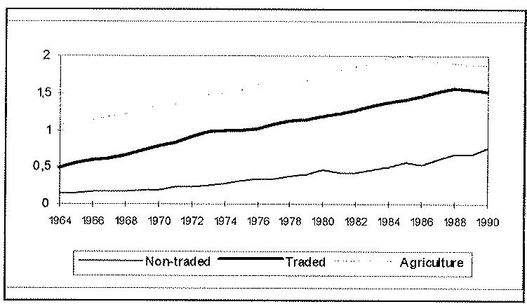
The implications of these changes for sectoral productivity in the three private sectors are apparent in Figure 2.1.2. As can be seen, there is a sharp increase in the labour productivity everywhere being particularly strong in the agriculture and manufacturing sectors.
Figure 2.1.1 : Sectoral Distribution of Employment.
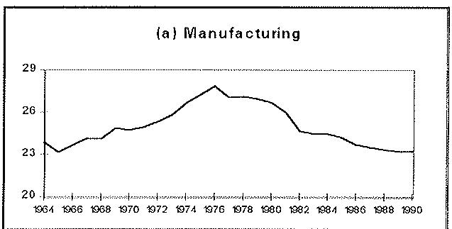
Percentage of total
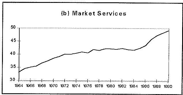
Percentage of total
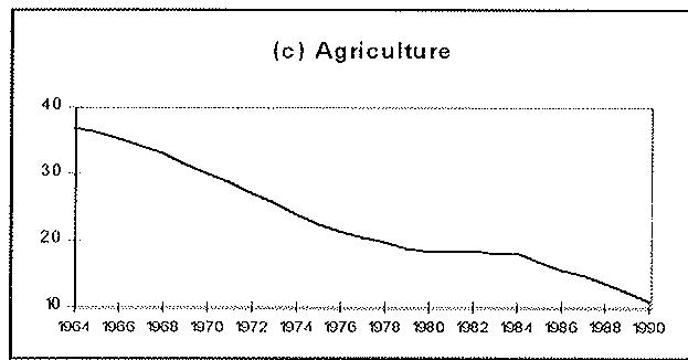
Percentage of total
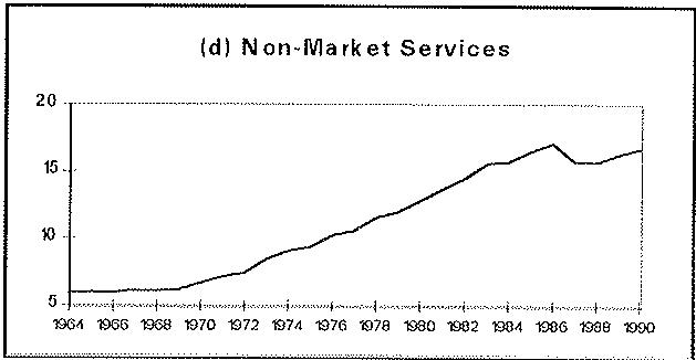
Percentage of total
Figure 2.1.2: Sectoral Productivity.
GDP per worker.
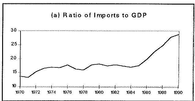
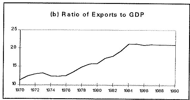
Figure 2.1.3, graphs (a) and (b), illustrates two measures of openness: the share of imports and exports in GDP, respectively. As can be seen, the Spanish economy has considerably increased its openness towards the rest of the world. There is, however, a significant change in this trend in the export share of GDP around 1985, remaining stable for the rest of the period. On the other hand, import share of GDP, accelerates it rise after 1985.
Figure 2.1.3: Openness.
Percentage of GDP
Percentage of GDP
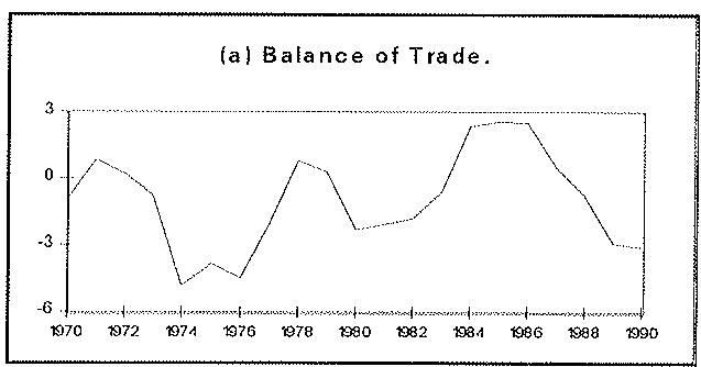
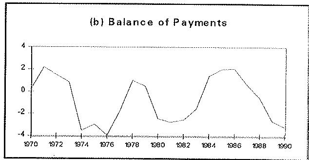
Related to openness is the balance of trade and the current account of the balance of payments, shown in Figure 2.1.4, graphs (a) and (b). As can be seen, the Spanish economy enjoyed a healthy trade position vis-à-vis the rest of the world between 1984 and 1986. For the most of the period, the trade deficit has been pronounced and has deteriorated since 1987. As a well-established feature of the external sector of the Spanish economy, both exports and imports are very responsive to the business cycle which makes the balance of trade to deteriorate rapidly during expansions and to improve during recessions.
Figure 2.1.4: Trade an International Payments Balance.
Percentage of GDP
Percentage of GDP
Figure 2.1.5: Public Expenditure and Taxation
Percentage of GNP
Percentage of GNP
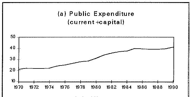
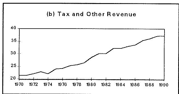
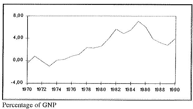
The rates of public expenditures and taxation are illustrated in Figure 2.1.5, graphs (a) and (b). As can be seen, there is a rapid growth in both expenditure and revenues, being former than in the latter reflecting, among other things, the countercyclical orientation of the budgetary policy and the consolidation of a democratic public sector. As a consequence of that unbalanced growth of expenditure and revenues, after 1975 the public sector borrowing requirements (shown in Figure 2.1.6), so far contained within narrow bands if not actually displaying a surplus, jumped rapidly to 7% of GDP between 1975 and 1985. After a period of reduction in the deficit, it continued to increase in 1989.
Figure 2.1.6: Public Sector Borrowing Requirement.
Percentage of GNP
Figure 2.1.7 shows the rapidly increasing gap that started to open between labour force and total employment since the early 1970s. Before that, the evolution of the unemployment rate was negligible. After the first oil crisis, it started to grow reaching two digit levels since 1980, peaking to 22% in 1985 and responding subsequently to the expansion, but never falling below 15%. The ongoing recession since 1992 has brought again to the forefront unemployment rate figures of 20%, revealing the extraordinary large hard core of unemployment present in the Spanish economy.
Figure 2.1.7: Unemployment Rate
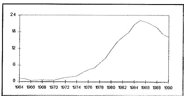
Percentage of Labour Force
Turning now to price and wage inflation, we show in Figure 2.1.8 the inflation rates of consumer prices (the deflator of private consumption) and the inflation rate of wages in the private sector. Although following a common trend during the 1965-90 period, prices peaked in 1977, while wages reached a peak in 1978. After the signing of the Moncloa Agreements in 1978, price-wages movements have been considerably closer than before, indicating that the indexation mechanism introduced since then has been helping wage moderation. In 1987 and 1989 the growth in wages was smaller than that in prices.
Figure 2.1.8: Price and Wage Inflation
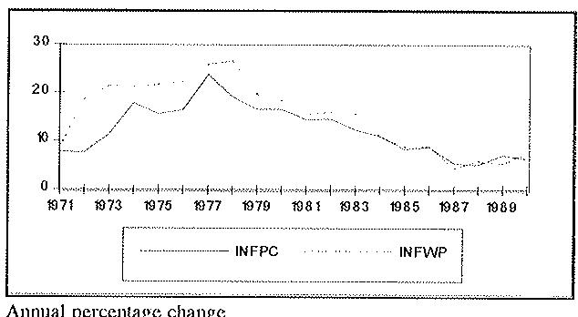
Annual percentage change
Finally, Figure 2.1.9 shows the growth rate of real GDP at factor cost. As can be seen, growth in GDP exceeded 5% in real terms in all except two years in the 1965-74 period, before dropping to 0.94% in 1975 in a delayed response to the 1973-74 oil price rises. Although growth recovered slightly in 1976-78, the second oil crisis in 1979 slumped GDP growth. After that, growth remained sluggish until 1986, averinging a mere 1% a year over the 1980-85 period. In 1986, the year Spain joined the EC, GDP growth increased to 2.5%, the largest push since 1977, reaching 5.7% in 1987, well above its European partners. After two more years of strong growth, GDP growth decelerated to 3.8% in 1990.
Figure 2.1.9: Growth Rate of GDP at factor cost
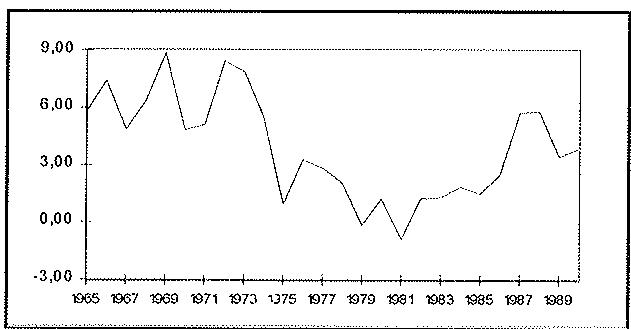
Annual percentage change
2.2. The Sectoral Breakdown
The HERMIN-Spain model has been conceived as a four sector model of the Spanish economy. The progressive sectoral breakdown for HERMIN-Spain is as indicated in the Table 2.1.
The choice of the sectoral disaggregation is justified by the desire of keeping the model as small and simple as possible while separating sectors with different behaviour and driven by different forces:
i) the public sector (G) is dependent on Government policy decisions, with expenditure and tax rates as instruments.
ii) the exposed tradable sector (T) is driven by both domestic and foreign demand, and by international cost competitiveness.
iii) the protected non-tradable sector (N) is driven by domestic demand, and
iv) the agricultural sector (A) is treated as mainly exogenous.
| Table 2.1 Sectoral breakdown in HERMIN-SPAIN | ||
| 2 Sectors | 3 Sectors | 4 Sectors |
| S1. Government (G) | S1. Government (G) | S1. Government (G) |
| S2. Private (P) | S2.1. Private Non Ag.(NA) | S2.1.1. Tradable (T): Industry |
| S2.1.2. Non Tradable (N): Energy, Building and Construction and Private Marketed Services | ||
| S2.2. Agriculture (A) | S2.2. Agriculture (A) | |
2.3. Key Aspects of HERMIN-Spain
In building the HERMIN-Spain model, we have opted for simple and encompassing theoretical foundations sufficiently established in other modelling exercises similar to this one. The way output, employment, wages, prices and aggregate demand are determined by the corresponding agents in the different sectors of the economy is explained in this chapter.
Taking into account that the model is going to be used for long-run policy analysis, the behaviour of the agents we are considering is not going to be affected by cyclical factors. This allows us to simplify further the specifications by just considering the fundamental determinants of the agents' decisions in agreement with the underlying theories. In what follows we will concentrate on the most important behavioural equations in HERMIN-Spain (see Herce and Sosvilla-Rivero, 1994b), listed in Table 2.2. The rest of the equations of the model can be found in Appendix 1.
2.3.1. The Behaviour of Firms
Only the tradable and non-tradable sectors are modelled behaviourally. The same CES production function is imposed in those sectors:
\[O = A \left\{\delta \left(\exp \left(\lambda_ {L} t\right) L\right) ^ {- \rho} + (1 - \delta) \left(\exp \left(\lambda_ {K} t\right) K\right) ^ {- \rho} \right\} ^ {- (1 / \rho)}\tag{2.1}\]
where O, L and K are, respectively, added-value, employment and the capital stock. A is a scale parameter, is the elasticity of substitution, is a factor intensity parameter and and are the rates of technical progress embodied, respectively, in labour and capital. Whenever is positive the technological progress will be factor saving.
In both T and N sectors, factor demands are derived on the basis of cost minimization subject to given level of output, yielding a joint factor demand equation system of the form:
\[\mathrm{K} = \mathrm{G} (\mathrm{O}, \mathrm{w/c})\tag{2.2}\]
and
\[\mathrm{L} = \mathrm{H} (\mathrm{O}, \mathrm{w/c})\tag{2.3}\]
where, c is the user cost of capital and w the wage rate.
Equivalently, by dividing by O, factor demands per unit of output can be expressed as:
\[\mathrm{K} / \mathrm{O} = \mathrm{g} (\mathrm{w} / \mathrm{c})\tag{2.2'}\]
and
\[L / O = h (w / c)\tag{2.3'}\]
Furthermore, in order to apply the estimation techniques to the existing data on employment and capital formation we take gross investment instead of the capital stock. The huge simplification this procedure entails can be justified assuming that the flow of gross investment is a proxy for the latest vintage of capital in a "putty-clay" world. Thus our final joint demand system will be:
\[\mathrm{I} / \mathrm{O} = \mathrm{g} (\mathrm{w} / \mathrm{c}); \text {with} \mathrm{g} ^ {\prime} > 0\]
and
(2.2')
\[\mathrm{L} / \mathrm{O} = \mathrm{h} (\mathrm{w} / \mathrm{c}); \text { with } \mathrm{h} ^ {\prime} < 0\tag{2.3"}\]
where I stands for gross investment.
Once it is computed, one can build a proxy for the capital stock following the perpetual inventory rule:
\[\mathrm{K} _ {t} = \mathrm{I} _ {t} + (1 - \alpha) \mathrm{K} (t - 1)\tag{2.4}\]
Given the cost minimization criterion adopted, we need an alternative determination of the level of output in every period in order to derive the levels of employment and investment.
The equation for output in the tradable sector is:
\[\mathrm{OT} = \mathrm{f} (\text { F D D W O T }, \mathrm{OW}, \text { C C O M P T })\]
where OT is the tradable sector added-value at factor cost, FDDWOT is a measure of final domestic demand where each of its components is weighted by their private domestic T sector added-value content, OW is a measure of world trade, and CCOMPT is a measure of relative (to the rest of the world) cost competitivenes in the tradable sector. CCOMPT is defined as follows:
\[\mathrm{CCOMPT} = \text { ULCT / ULCEC11 }\tag{2.5}\]
where ULCT are nominal labour costs in the tradable sector and ULCEC11 are nominal (in pesetas) unit labour costs in the European Community countries except Spain, weighted by their share of total GDP.
Equation (2.5) was estimated including a time trend to account for variations in the weights used in composing FDDWOT. From the estimated equation, the long-rung elasticities of T sector output with respect to final domestic demand weighted by T sector output content, world output and expected cost compentiniviness are 0.57, 0.64 and -0.50, respectively.
Output in the non-tradable sector (ON) is assumed to be demand driven, the driving variable being final demand where its components are weighted by their private domestic N sector added-value content (FDWONO), treating investment in building and construction independently (IHIBC):
\[\mathrm{ON} = \mathrm{f} (\text { FDWONO }, \text { IHIBC })\tag{2.6}\]
Estimation of equation (2.6) yields the following coefficients for IHIBC and FDWONO: 1.00 and 0.47, respectively.
Concerning the estimation of the parameters of the CES production function in the T and the N sectors, Table 2.3 summarises the estimated parameters.
| Table 2.3 The CES Technology: T and N sectors | |||
| Parameter | T-Sector | N-Sector | Description |
| σ | 0.7750 | 0.5105 | Elasticity of Substitution |
| $λ_{L}$ | 0.0371 | 0.0226 | Rate of Technical ProgressEmbodied in Labour |
| $λ_{K}$ | -0.0687 | 0.0276 | Rate of Technical ProgressEmbodied in Capital |
| δ | 0.9783 | 0.9924 | Factor Intensity Parameter |
| A | 0.6882 | 1.1733 | Scale Parameter |
Notice technical progress is estimated to be capital using and labour saving in the T sector at a rate of 6.9 and 3.7 percent per annum, respectively, whilst in the N sector it is estimated to be both capital and labour saving, at a rate of 2.8 and 2.2, respectively.
As mentioned above, the agriculture sector is treated separately as mainly exogenous, being the public sector also handled mainly through exogenous policy instruments.
2.3.2. Wage Determination and Wage Bargaining
Wages result out of a process of wage bargaining between employers and trade unions. Of the very many elements that are relevant in this process [Nickel, Layard and Jackman (1986); De Lamo y Dolado (1993)] we will only consider consumption prices, productivity of labour, the unemployment rate and the tax wedge.
In the bargaining process, unions will, above all, try to translate price and productivity increases into nominal wages and, as long as they realize them fully, do the same with all kind of taxes that diminish their disposable income and/or its purchasing power. In doing so they will be restrained by the state of the labour market reflected in the current unemployment rate or its rate of change. Clearly, their power in the negotiation will be endangered by an excessive unemployment level. This is the so-called "Phillips curve" effect.
The proposed equation for the determination of wages, consistent with the above description of the bargaining process will thus be:
\[\mathrm{W} = \mathrm{f} (\mathrm{PC}, \mathrm{PROD}, \mathrm{UR}, \mathrm{WEDGE})\tag{2.7}\]
where PC is the private consumption deflator, PROD is the productivity of labour obtained as real output over employment in the corresponding sector, UR is the percentage unemployment ratio and WEDGE is the ratio of (1 + the indirect implicit tax rate) over (1 - the direct implicit tax rate) (inclusive of social contributions).
Estimation of equation (2.7) for the T sector shows a change in the elasticity of wages in that sector with respect to consumption prices after the Moncloa Agreements: before 1978 there was a strict over-indexation of wages to prices, and after that year an under-indexation. The estimated equation suggests that productivity gains are not fully translated into wages, since its coefficient is 0.70. The Phillips curve effect (-0.005) is roughly half the size to that reported for Spain in Drèze and Bean (1990, p.23), and also much smaller than those obtained for Ireland (-0.026) [Bradley and Wright, (1994)] and Portugal (-0.046) [Modesto and Neves, (1993)]. Finally no significant tax-wedge effect is found, but we find a significant and negative effect for a dummy variable proying Spanish integration into the EC, that could be driving by the removal of trade barriers after entry in to the Community.
Estimation of equation (2.7) for the N sector also shows a change in the elasticity of wages in that sector with respect to consumption prices after 1978: before that year there was over-indexation of wages, and after that year under-indexation. The estimated equation suggests that productivity gains are more than fully translated into wages, being its coefficient of 1.40. The Phillips curve effect (-0.006) is greater than that estimated for the tradable-sector wages. Finally no significant tax-wedge effect was found.
In the government and in the agricultural sectors, wages will simply be assumed as following wage setting patterns in the T sector.
2.3.3. Price Determination
Producer prices in the T and N sectors are determined as a markup on unit labour costs. In the case of the price of the T sector output, the world price also plays a role.
The majority of absorption deflators (PABS) are modelled in the following way:
\[\log (\mathrm{PABS}) = a _ {0} + a _ {1} \log (\mathrm{PGDPFC}) + (1 - a _ {1}) \log (\mathrm{PMP})\]
where PGDPFC is the deflator of total GDP at factor cost and PMP is the deflator of total imports. Exposure to competition at home and abroad will determine the weights in this combination. The only exceptions in this general approach are the consumption deflator (PC), where we add a term to account for the influence of net indirect taxes (TINC) on consumer prices, the price of public consumption, the price of exports of turistic and non turistic services and the price of residential investment, where no significant effect was found for PMP.
2.3.4. Labour Force Participation
The extent to which the working age population (N1564, or total population of age between 15 and 64 years old) opts for participating into the labour force (LF) depends, leaving apart demographic factors captured here by a time trend, on the situation of the labour market given by the unemployment rate. In a rather simplistic way, thus, we will represent the labour supply by the following set of equations:
\[\mathrm{LFPRF} = \mathrm{f} (\mathrm{UR}, \text { time })\tag{2.8}\]
\[\mathrm{LFPRM} = \mathrm{f} (\mathrm{UR}, \text { time })\tag{2.9}\]
\[\mathrm{LFPR} = \mathrm{LFPRM} + \mathrm{LFPRF}\tag{2.10}\]
\[\mathrm{LF} = \mathrm{LFPR} * \mathrm{N1564}\tag{2.11}\]
\[\mathrm{UR} = 1 0 0 ^ {*} ((\mathrm{LF-L}) / \mathrm{LF})\tag{2.12}\]
where LFPRF, LFPRM and LFPR are female, male and total labour force participation rates respectively, UR the unemployment ratio, time a time trend, and L employment. The effect of UR on the participation rates, the encouragement effect, should have a negative sign [as established by several authors -see e.g., De Hevia and Novales, (1992)], that is, the greater UR, the lower LFPRF or LFPRM. No sectoral breakdown is adopted for this part of the model.
The estimated equations show a greater effect of unemployment on the participation ratio for women than for men (-0.002 and -0.001, respectively). The time trend only appears to be significant in the female labour force participation rate, and of the expected sign.
2.3.5. Private Consumption
Consumption by households is the largest single item in aggregated demand. A liquidity constrained consumption function is used, linking private consumption to real personal disposable income and real financial wealth.
\[\text { The consumption function is thus: }\]
\[\mathrm{CONS} = \mathrm{f(YRPERD,GNDD/PC)}\tag{2.13}\]
where YRPERD is real personal disposable income (see Appendix 1 for a precise definition of how it is derived) and GNDD/PC is the outstanding debt of the government held by domestic residents, in real terms (as a proxy for financial wealth).
We obtain an estimated marginal propensity to consume of 0.94, which implies a marginal propensity to save of 0.06 and a conventional weath effect of about 0.04.
2.3.6. Total Investment
The way factors demand were estimated saves us the separate specification of a private non residential investment equation. Total (gross) fixed investment, I, results out of the following identity:
\[\mathrm{I} = \mathrm{IP} + \mathrm{IH} + \mathrm{IG}\]
\[\mathrm{IP} = \mathrm{IT} + \mathrm{IN} + \mathrm{IA}\tag{2.14}\]
(2.15)
where IP is gross fixed private non residential investment; IT, IN and IA is the split of IP between the tradable, non-tradable and the agricultural sectors; IH is the gross fixed private residential investment; and IG is gross fixed public investment (an exogenous variable).
Residential investment, IH, is a function of personal disposable income, YRPERD, both expressed in per capita terms:
\[\mathrm{IH} / \mathrm{N} 1 5 6 4 = \mathrm{f} (\text { Y R P E R D } / \mathrm{N} 1 5 6 4)\tag{2.16}\]
The estimated elasticity of IH with respect to YRPERD is 0.86.
2.3.7. Imports, Exports and the Balance of Trade
In order to assure the closing of the model it was decided that imports should not be modelled behaviourally but rather determined residually once output and exports had been estimated (see Appendix 1 for details). Exports in the private sector, XP, are:
\[\mathrm{XP} = \mathrm{XT} + \mathrm{XN} + \mathrm{XA}\]
that is, exports in the T sector, XT, exports in the N sector, XN, and agricultural exports, XA.
Agricultural exports (XA) are estimated as a ratio to agricultural output against a constant and a time trend.
It is well known [see, e.g., Fernández and Sebastián, (1991)] that industrial exports in Spain increase when domestic producers find difficulties to sell their products at home.
Manufacturing sector exports (XT) are thus estimated as follows:
\[\mathrm{XT} = \mathrm{f} (\mathrm{OW}, \text {GNPDOT}, \text {CCOMPT}, \text {DUMCEE})\]
that is, XT is a function of world output, the rate of growth of gross national product (proying the economic cycle), cost competitiveness, and a dummy variable to take account of the joining of Spain to the European Community in 1986 since this fact changed the trade regime of the Spanish economy. The estimated coefficients are 1.63, -1357.47, -28.62 and -476.20, respectively.
Exports of the N sector have been split into tourism exports (XTUR) and non-tourism ones (XNTUR). The former are assumed dependent of world output and (cost) competitiveness, and the latter only of world output. Indeed, touristic exports are known to be highly dependent on the western economies cycle. The estimated elasticity of XNTUR with respect to world output is 0.91 whilst the elasticities of XTUR with respect to world output and cost competitiveness are 1.05 and -1.16, respectively.
The high income elasticity of Spanish imports is also well documented [see, e.g., Sebastián (1991)]. This fact is properly captured by the way imports are residually determined in HERMIN-Spain.
2.3.8. Income Determination Behavioural Equations
There are only two estimated equations in the income determination part of the model: total depreciation and undistributed profits. The rest of the magnitudes are derived through identities (see Appendix 1).
i) Total depreciation:
Total depreciation (DEP) is determined in a "technical" relation as a function of the value of total private capital stock (PIP*KP). The estimated short-run elasticity is 0.39, being the long-run elasticity 0.98.
ii) Undistributed profits:
Undistributed (i.e. retained) profits (YCU) are cyclically influenced by the growth rate of GNP (GNPDOT) and by total profits (YC), being the estimated coefficients 0.02 and 1.11, respectively.
Notice that these results imply that the undistributed profits increase both as company income rises and during recoveries.
3. The Spanish CSF 1994-99
This section documents the total financial endowments of the Spanish CSF for the 1994-99 period distinguishing by functional sector of destination and institutional sector of origin. It also contains an estimation of the likely expenditure shock to the beneficiary regions and a summary description of these.
To date, the Spanish authorities are still negotiating the CSF amounts for the Objective no. 2 regions and their figures are not yet available. These amounts, however, are reduced as compared to those already approved for the rest of the Objectives-regions. In this exercise thus, we will be dealing with the amounts stemming out of the Spanish Regional Development Plan [PDR (1994)] submitted by the Ministry of Finance to the EU Commission within the CSF negotiating procedure and finally approved by Brussels.
Spain is the major recipient of CSF grants of Community origin. However, not all its regions are eligible for them. Of the seventeen Comunidades Autónomas, plus the towns of Ceuta and Melilla in the North-African coast, only ten and the two beforementioned towns are elegible. This obliges our macroeconomic exercise to a complementary assessment that, nevertheless, will not be attempted here but in the near future. Section 3.3, below, contains some thoughts on this issue.
The total Spanish CSF funds for the 1994-99 period amount to 48.9 bn ECU at 1994 prices of which, on average, the EU contribution will be 67.3%. In annualized terms, this is equivalent to almost 2% of the Spanish GDP estimated for 1994 although some regions will have much larger figures. These regions are the less developed according to the Structural Funds criteria, basically GDP per head relative to the Union's average. These regions have also higher unemployment ratios and lower infrastructural endowments.
3.1. The financial conventions of the CSF 1994-99 and their sectoral breakdown
CSF expenditures are directed towards three major areas: physical infrastructure, human resources and aids to production and firms. The CSF or Community Support Framework is, however, nothing but the "financial envelope" of a series of operational programmes grouped under the umbrella of the Regional Development Plan or RDP. The RDP is thus the operational pillar of the EU's regional policy while the CSF is its financial pillar or the counterpart of the RDP.
Every funded intervention of the CSF must be integrated within an operational programme. Typically, the CSF consists of several hundreds of such interventions, and their corresponding financial plans, ranging from transport infrastructure projects to funding for the provision of hospital equipment. These interventions are funded both by the EU and by the recipient member State and, as for the last share, all public administrations as well as public and private firms may intervene.
Within the three major categories of expenditure first mentioned, there exists also a detailed breakdown according to the sector to which they are directed. Table 3.1 shows the sector/subsector details and the origing of funds.
| Table 3.1Spanish CSF 1994-99 Funds: Distribution by Sector (bn. ECU 1994) | |||||||||
| CSF sector/subsector code | EU funds | EU funds % of (1) | Gov. funds | Gov. funds % of (1) | Total public funds (1) | Private invest. | Private invest. % of (2) | Total CSF funds (2) | Share of each sector in (2) |
| 1. Physical infrastructure | 11250.4 | 61.6 | 7001.8 | 38.4 | 18252.1 | 0.0 | 0.0 | 18252.1 | 37.3 |
| Transport | 6099.7 | 64.6 | 3339.0 | 35.4 | 9438.6 | 0.0 | 0.0 | 9438.6 | 19.3 |
| Energy | 623.8 | 40.0 | 935.7 | 60.0 | 1559.4 | 0.0 | 0.0 | 1559.4 | 3.2 |
| Communications | 417.9 | 35.0 | 776.2 | 65.0 | 1194.1 | 0.0 | 0.0 | 1194.1 | 2.4 |
| Environment | 3034.0 | 68.3 | 1406.4 | 31.7 | 4440.4 | 0.0 | 0.0 | 4440.4 | 9.1 |
| Water resources | 1303.4 | 65.7 | 680.8 | 34.3 | 1984.3 | 0.0 | 0.0 | 1984.3 | 4.1 |
| Environmental conservation | 1730.5 | 70.5 | 725.6 | 29.5 | 2456.1 | 0.0 | 0.0 | 2456.1 | 5.0 |
| Health equipments | 452.3 | 60.7 | 292.6 | 39.3 | 744.8 | 0.0 | 0.0 | 744.8 | 1.5 |
| Education equipments | 622.8 | 71.2 | 252.0 | 28.8 | 874.8 | 0.0 | 0.0 | 874.8 | 1.8 |
| 2. Human Resources | 6276.8 | 75.1 | 2084.0 | 24.9 | 8360.9 | 29.3 | 0.3 | 8390.1 | 17.2 |
| Specific training needs for industry | 126.3 | 75.0 | 42.1 | 25.0 | 168.4 | 0.0 | 0.0 | 168.4 | 0.3 |
| Specific training needs for tourism | 11.8 | 75.0 | 3.9 | 25.0 | 15.8 | 29.3 | 65.0 | 45.0 | 0.1 |
| Specific Training for R&D | 164.5 | 75.4 | 53.7 | 24.6 | 218.2 | 0.0 | 0.0 | 218.2 | 0.4 |
| Occupational training | 1602.3 | 74.6 | 546.7 | 25.4 | 2149.0 | 0.0 | 0.0 | 2149.0 | 4.4 |
| Permanent training | 460.5 | 75.3 | 151.2 | 24.7 | 611.7 | 0.0 | 0.0 | 611.7 | 1.3 |
| Employment promotion | 3322.3 | 75.4 | 1085.4 | 24.6 | 4407.7 | 0.0 | 0.0 | 4407.7 | 9.0 |
| Specific measures for long-term unemp. | 589.2 | 74.6 | 201.1 | 25.4 | 790.3 | 0.0 | 0.0 | 790.3 | 1.6 |
| 3. Production aids | 8584.5 | 70.4 | 3605.1 | 29.6 | 12189.7 | 9824.2 | 44.6 | 22013.8 | 45.0 |
| To A sector | 3234.0 | 72.1 | 1252.5 | 27.9 | 4486.5 | 961.8 | 17.7 | 5448.2 | 11.1 |
| Agriculture, rural dev. and fisheries | 3234.0 | 72.1 | 1252.5 | 27.9 | 4486.5 | 961.8 | 17.7 | 5448.2 | 11.1 |
| To T sector | 2467.1 | 70.5 | 1034.2 | 29.5 | 3501.2 | 3834.8 | 52.3 | 7336.0 | 15.0 |
| Food industry | 1220.0 | 70.0 | 522.9 | 30.0 | 1742.9 | 1200.0 | 40.8 | 2942.9 | 6.0 |
| Other industry | 1005.7 | 70.9 | 413.0 | 29.1 | 1418.7 | 2634.8 | 65.0 | 4053.5 | 8.3 |
| Industrial estates | 241.4 | 71.1 | 98.3 | 28.9 | 339.6 | 0.0 | 0.0 | 339.6 | 0.7 |
| To N sector | 2883.5 | 68.6 | 1318.5 | 31.4 | 4202.0 | 5027.7 | 54.5 | 9229.6 | 18.9 |
| Local dev. and services to firms | 1646.1 | 70.6 | 685.7 | 29.4 | 2331.7 | 4288.1 | 64.8 | 6619.8 | 13.5 |
| Aids to tourism | 245.4 | 61.6 | 152.8 | 38.4 | 398.2 | 739.6 | 65.0 | 1137.8 | 2.3 |
| Resources touristic/interest | 292.1 | 60.9 | 187.9 | 39.1 | 480.0 | 0.0 | 0.0 | 480.0 | 1.0 |
| Aids to R&D | 699.9 | 70.6 | 292.1 | 29.4 | 991.9 | 0.0 | 0.0 | 991.9 | 2.0 |
| 4. Miscellaneous | 188.3 | 75.7 | 60.4 | 24.3 | 248.7 | 0.0 | 0.0 | 248.7 | 0.5 |
| Monitoring, assistance and guidance | 188.3 | 75.7 | 60.4 | 24.3 | 248.7 | 0.0 | 0.0 | 248.7 | 0.5 |
| Total | 26300.0 | 67.3 | 12751.3 | 32.7 | 39051.3 | 9853.4 | 20.1 | 48904.7 | 100.0 |
| Source: Spanish Ministry of Finance. One ECU in 1994 amounts to 155 Pta. | |||||||||
One thing to be noted is that private expenditure makes part of the Total CSF funds on top of EU and national public funds. This private expenditure is assumed by the CSF authorities to accompany public aids to production, very often as a requirement for the last to be agreed to firms. As for the total CSF public funds, expenditure on physical infrastructure represents 46.7% of the total, expenditure on human resources 21.4% and production aids 31.3%.
Physical infrastructure
Half of the expenses under this heading are devoted to transport infrastructure of all kinds and one fourth of those to environmental infrastructure aimed at the water cycle and conservation of the environmental resources. The rest of the expenses are apportioned equally to energy and communications infrastructure and to health and education equipment.
The strategic objectives of the interventions under this expenditure chapter are the articulation of the territory, improved accessibility for isolated rural areas, improvement of urban transport and coherence of all transport modes in what concerns transport infrastructure.
The water cycle in Spain is very distorted by the unbalanced distribution of supply and demand of the resource and the considerable margin existing for a complete treatment of the used resource. Many other aspects of catastrophic nature are associated to the water cycle in Spain that have consequences for the environment. Their consideration in an integrated way under the strategy of the operational plans is clearly an opportunity for improvement with additional beneficial consequences for the economy.
Specific environmental action aims at comprehensive wastage treatment, the restoration of damages caused by public works, restoration of beaches and coasts and forest fire prevention. However, the environmental dimension of many of the water-cycle interventions must not be forgotten.
Concerning telecommunications, the aims are to catch-up with the Unions's average indicators in this matter, the universalization of basic communications service and the renewal of the technology of the infrastructure. It is also envisaged the gradual introduction of the new technologies and services in this field and its extension to the less developed territories.
In the energy field the strategic objectives are efficiency, security and diversification. The environmental dimension is not forgotten in the provisions of the corresponding operational plans.
The health and education equipments considered try to rebalance the relatively low endowment of this kind suffered by the objective number 1 regions contributing thus to solve the excess demand present in these regions.
Human resources
Expenses under this line, half of the total, are devoted mostly to employment promotion through the removal of the thousand obstacles to mobility, adequate skills, stable employment opportunities, etc. The improvement of occupational training schemes is also an important priority that absorbs one fourth of expenses devoted to human resources. In this area, the CSF interventions will reinforce the national plans already under way. Besides that, there are specific measures directed towards permanent training in the workplace, the long term unemployed, training needs for certain industries and trades, tourism, R&D, etc.
Aids to production
This chapter is very important in the new Spanish CSF for the 1994-99 period. It absorbs a larger share of total CSF expenditure than the previous one and is roughly equally distributed amongst the three private sectors of the HERMIN-Spain model: agriculture (37%), manufacturing (29%) and services (34%).
Each sector has, according to the operational plans, an specific approach given their particular starting point.
The agricultural sector requires considerable rationalization and diversification efforts, productivity enhancement and accompanying measures to ensure an easy transition towards more productive and less labour intensive units.
Industry in Spain faces severe problems of upgrading, internationalization and critical size. SMEs are very numerous and their problems are also specific lacking, in particular, proper assistance and general services directed to them. Industry related to the agricultural products has an important potential but the problems just mentioned are particularly acute in this sector.
Among services, the provision of all kind of technical assistance and general services to firms, as mentioned in the previous paragraph, needs to be considerably developed so that, not surprisingly, this is the major priority of aids to this sector. Touristic services and the associated resources are also targeted by the CSF interventions. Finally, R&D activities result favored as well.
3.2. The CSF expenditure shock to the regional economies
At present, only 33% of total CSF expenditure can be properly attributed to specific regions. The rest of the expenditure remains "pluri-regional" and the data we are using does not allow a precise distribution across regions. However, assuming a simple rule of distribution based in the actual distribution of the regionalized expenditure one can obtain an estimate of the expenditure shock that the CSF represents for the objective number 1 regions. This is done in Table 3.2.
The first column of the table shows the distribution of total CSF funds by region (ten + Ceuta and Melilla). Assuming, next, a uniform distribution of expenditures across time, we defined the annualized CSF expenditure by region and compare it to the estimated 1994 regional GDP (in fact Gross Value Added, see notes to the table for a description of its estimation). It can be seen that, as a percentage of regional GDP, annualized CSF expenditure amounts to almost 2% of the former for the whole country, while the regional figures are much higher on average ranging from 2.14% for the Comunidad Valenciana to 8.15% for Extremadura. The last is probably too high and due to the simple assumptions made for the distribution of pluri-regional expenditure.
From a macroeconomic point of view, such a percentages represent similar shocks to aggregate expenditure, well above the conventional sizes used in policy simulations. Their demand effects will be correspondingly high.
| Table 3.2CSF Funds and Regional GDP in Objective No. 1 Regions | ||||
| CSF 94-99(a) | Annualized CSF 94-99(a) (b) | Regional GDP 94(c) | Annualized CSF as % of Regional GDP | |
| Andalucía | 13778.64 | 2296.44 | 53425.30 | 4.30 |
| Asturias | 1949.83 | 324.97 | 10476.95 | 3.10 |
| Castilla y León | 6435.78 | 1072.63 | 24692.66 | 4.34 |
| Castilla La Mancha | 4207.45 | 701.24 | 14353.27 | 4.89 |
| Canarias | 3157.47 | 526.25 | 15834.11 | 3.32 |
| Cantabria | 919.99 | 153.33 | 5355.09 | 2.86 |
| C. Valenciana | 5718.39 | 953.07 | 44535.67 | 2.14 |
| Extremadura | 3678.26 | 613.04 | 7521.47 | 8.15 |
| Galicia | 6913.40 | 1152.23 | 24562.85 | 4.69 |
| Murcia | 1928.00 | 321.33 | 9432.78 | 3.41 |
| Ceuta y Melilla | 217.52 | 36.25 | 951.49 | 3.81 |
| Spain | 48904.75 | 8150.79 | 429153.60 | 1.90 |
| Notes: amounts are in 1994 million ECU(a) Non regionalized CSF funds have been attributed to regions according to their share in total regionalized funds(b) Total CSF funds have been equally attributed to each year(c) Regional GDP has been estimated assuming a cumulative nominal 5% growth per year applied to the 1992 figure for each region obtained from Alcaide (1993)Sources: Spanish Ministry of Finance, Alcaide (1993) and own computations. | ||||
3.3. The Spanish Objective no. 1 regions and the likely regional effects of the CSF
The reform of the EU Structural Funds establishes several major objectives under which regions or territories are elegible for structural aids. The objective no. 1 envisages the less-developed regions of the Union considering as such those regions whose GDP per head is below 75% of the Union's average. Ten Spanish regions have their GDP per head under this line, together with the towns of Ceuta and Melilla in the North-African coast. They are listed in table 3.3 together with some selected indicators of their relative position within the national context.
| Table 3.3Summary Indicators for Spanish Ob. No. 1 Regions | |||
| GDP per head (1992) | Unemployment (1993) | General Infrastruct. endowment (1990) | |
| Andalucía | 69.6 | 33.0 | 103.2 |
| Asturias | 87.2 | 20.6 | 96.3 |
| Castilla y León | 88.0 | 20.2 | 93.2 |
| Castilla La Mancha | 78.4 | 19.5 | 67.7 |
| Canarias | 95.7 | 28.4 | 83.3 |
| Cantabria | 92.2 | 19.8 | 84.0 |
| C. Valenciana | 104.6 | 23.7 | 109.8 |
| Extremadura | 64.2 | 29.9 | 70.0 |
| Galicia | 81.7 | 18.0 | 90.6 |
| Murcia | 81.5 | 24.9 | 83.0 |
| Ceuta y Melilla | 69.3 | 24.5 | n.a. |
| Spain | 100.0 | 21.5 | 100.0 |
| Sources: Alcaide (1993), EPA (1994), Cutanda y Paricio (1992) and own computations. | |||
Taking into account that the Spanish GDP per head of population was, in 1992, about 71% of the Union's average, one can see that all the regions listed in the table fulfil the criterion previously stated, even if their GDP per head is above the Spanish average. Regions like Extremadura or Andalucía have their GDP p.h. index below 50% of the Union's average.
Unemployment is also very high in some of these regions and their general infrastructural endowment, relative to the national average, is generally lower as well.
These regions are thus the major beneficiaries of the CSF package. One thing is, however, that the regional economies receive such an important shock and another is that they are in a position to fully collect the potencial benefits of the structural measures taken. In this respect, the microeconomic and multi-criterium evaluation of the proposed measures is of paramount importance.
The Commission of the EU is constantly pushig for this type of exercise to be undertaken but there is no obvious way to do it given the complexity of the CSF. An attempt has been made by a large team coordinated by one of the authors [Herce et al. (1994)] to develop such a methodology, basically consisting in field work upon a selected sample of the 1989-93 CSF interventions and the use of Input/Output and pannel data regression techniques.
The preliminary results of this exercise show that the CSF has the potential to provoke structural change and economic integration with the rest of the territory in these regions as long as the interventions have the "appropriate" size and strategic nature. The planning process has been careful and realization of the works has been kept reasonably within time and budget. This ensures that the starting point of the long term effects is satisfactory. During the period of realisation, the use of local resources, labour and other inputs, has been intense and thus the generation of value added.
The future operation of the "new capacity" allowed by the CSF interventions has yet to be checked concerning the efficiency with which it is used, the priority of the purposes to which it is assigned and the decisions taken by the private agents to which the interventions are aimed at. Those conditions are precisely what allow the CSF "long-term growth crop" to be collected.
4. The Macroeconomic Effects of the CSF
This section deals with the conceptual issues arising out of the need to fully incorporate, into a macroeconomic framework, the presumed effects of an expenditure package like the CSF, aimed at substancial structural change of the beneficiary sectors. In this respect, the lack of microeconomic or sectoral evidence is particularly disturbing because the best way to capture structural change within a macroeconomic model is to calibrate its production side with parameters whose values have been previously computed based on that evidence.
4.1. A Diagrammatic Representation of the Supply and Demand Effects of the CSF
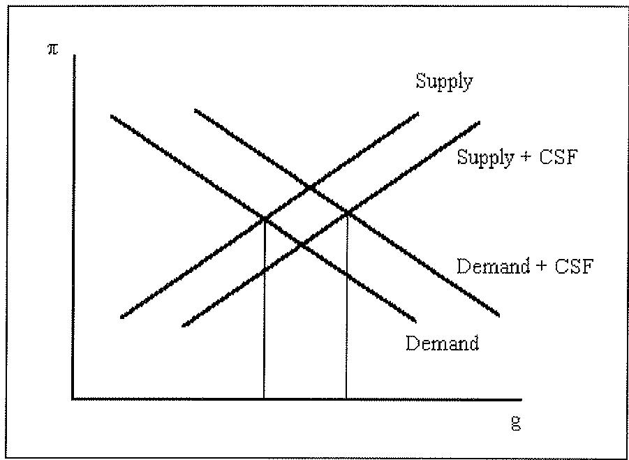
With the help of the text-book diagramme of Figure 4.1 it can be seen that CSF expenditure may have two types of effects.
First, the conventional Keynesian shock to aggregate demand will shift the demand curve to the right provoking higher inflation and higher growth. On the other hand, in as much as structural spending diminishes costs, increases productivity, allows differentiation of products, concentration of activities, etc. the supply curve will shift down reflecting the improved costs conditions of firms.
Altogether, the above supply and demand shocks would have a reinforced growth effect, while the inflationary pressures induced by the demand shock would be alleviated by the costs reductions due to the supply shock. This simple representation, however, should not help to hide the fact that supply effects take time and require a bunch of favourable conditions beyond the control of policy makers.
4.2. The supply Effects of CSF: the Role of Externalities
Providing more and better infrastructure or increasing the quality of the labour force or even granting structural aids to firms may decisively contribute to improve the cost conditions of large groups of industries in certain sectors or territories. Very often these activities act as if private firms were enjoying the use of additional productive factors at no cost, alternatively they may help to make the current inputs firms are actually using available at a lower cost or, finally, the general conditions under which firms operate result improved as a consequence. In all these ways, as Meade (1952) made eloquently clear, positive externalities may arise out of structural interventions. These are our supply shocks of the previous section.
The literature on the aggregated effects of infrastructure on growth, productivity and costs points towards substantial effects although these may be smaller at the regional level. However, externalities seem to have a higher impact in less developed regions [see Aschauer (1989), Munnell (1992) and, for a survey of the related literature, Draper y Herce (1993). Bajo-Rubio y Sosvilla-Rivero (1993) and Argimón et al. (1993) have treated the Spanish case].
The way HERMIN type models deal with externalities is developed in Bradley et al. (1994). Their approach is adopted here in section 5.1 below.
Infrastructural investment does reduce unit costs and increases the productivity of private factors of production through the scale and technological parameters of the production function. It also contributes to the attractiveness of the territories it affects for external private investment and increases the potential for agglomeration, provided other conditions exist.
Human capital investment shows up in the labour embodied technical progress rate directly increasing the productivity of this factor through the requirements of less amounts of efficient employment per unit of output. The eventuality of less physical labour needed per unit of output is particularly acute in this case but is also present in the other cases. Employment can thus actually increase after an externality creating shock if income and output effects are sufficiently large.
Aids to private firms will contribute to lower the user cost of capital although they may affect also to other inputs, energy or labour in particular. Amongst them, aids to R&D activities or the creation of industrial sites may have important consequences towards improving the environment in which activities take place putting the incumbent firms, or other firms newly attracted to the area, into a better position to compete in internal and external markets, through conventional or intra-industry trade relationships. These actions are particularly suited for the promotion and upgrading of conventional activities and the renewal of a region's sources of competitive advantages.
4.3. Externalities and Trade
As we have seen, some of the long-term effects of the CSF may have consequences for the upgrading of sectors and the attractiveness of territories. According to the recent literature on economic geography [see Krugman (1991a,b) and Krugman and Venables (1993)], the concentration and agglomeration trends should increase with the deepening of the EU internal market and the post-Uruguay Round process.
On the one hand, the reform of the Structural Funds by the EU, in 1987, was claimed by the peripheral members of the Union as a compensating response to the adverse shocks these could suffer because of the internal liberalisation. On the other hand, given the importance and the specific targeting of the CSF measures, beneficiary countries and regions may actually profit for placing themselves within the above mentioned trends and processes. We have attempted, in a very simplistic way, to introduce these effects through an increase in world demand for Spanish manufactures (see section 5.1 below).
Of course, when discussing about competitive advantages and the way their sources may be renewed, it is important to notice that many factors need to operate simultaneously. The diagramme in Figure 4.2, adapted from the discussion in Krugman and Venables (1993), is but a simplified representation of the many and complex interactions at work, not easily found, however, in backwarded regions.
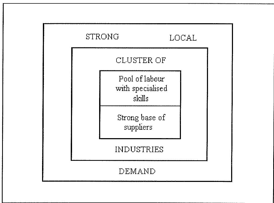
Not surprisingly, human capital is in the hard core of the clustering process. Infrastructure for transport and, increasingly, the communications must also be because of the crucial role it plays in linking any firm with its suppliers and its customers. Indeed, recent studies [Martin and Rogers (1993a)] confirm the role played by all these factors. Moreover, these studies [Martin and Rogers (1993b), Krugman and Venables (1993)] show the ambiguous pattern of benefits that increasing economic integration may have on the concerned territories. It is thus likely that CSF interventions would help the beneficiary regions and countries to participate actively in the distribution of benefits that arise out of deeper economic integration [see Emerson et al. (1988), Baldwin (1989) and OCDE (1993) for sharp assessments of these benefits].
5. Incorporating The CSF into the HERMIN Model
In this section we briefly describe our approach to the quantification of the medium to long-term impacts of the CSF 1994-99 on the Spanish economy using the HERMIN model. We first set out the way in which the CSF is incorporated into the model, using simple approximations that capture the broad thrust of the size and nature of the main expenditure programmes. We then illustrate the operation of the CSF mechanism included in HERMIN-Spain, using for the purposes of exposition a sequence of stylised simulations based on the infrastructural components of CSF. The aim of this exposition is to motivate the subsequent examination of the actual CSF, where we analyse the consequences for the Spanish economy (section 6), followed by a comparison with the CSF effects on the Irish and Portuguese economies (Section 7), and to define some model-based notation and terms.
5.1 Incorporating The CSF into the HERMIN
As mentioned above, there are three main economic channels through which CSF will influence on peripheral economy's long-run supply potential:
(i) through increased investment designed to improve physical infrastructure,
(ii) through increases in human capital, due to investment in human resources, and
(iii) through direct assistance to the private sector to stimulate investment, thus increasing factor productivity and reducing sectoral costs of production.
Let us examine three mechanisms in turn, briefly outlining how each of them are incorporated in the HERMIN model.
5.1.1 Physical infrastructure
Infrastructural investment takes a number of forms. It is the potential improvements to the efficiency of the supply side of the economy that infrastructural investment can be expected to have its main long-term impact. Our analysis takes a somewhat experimental approach to quantifying these supply-sides.
Within the HERMIN model an increase in the stock of physical infrastructure (over a baseline, no-CSF level) is assumed to benefit the supply side of the economy through the externality mechanisms described in Section 4. Such beneficial externalities lead to an increase in factor productivity and output capacity as well as a reduction in the costs of production.
Our model assumes that any CSF-based expenditure in infrastructure that is directly financed by UE aid subvention, IGVCSFEC, is matched by domestically financed expenditure of IGCSFRAT*IGVCSFEC, where IGCSFRAT is the domestic public co-financing ratio to be derived from Table 3.1. Hence, the total public expenditure is defined in the model as follows:
\[\mathrm{IGVCSF} = (1 + \text { IGCSFRAT }) ^ {*} \text { IGVCSFEC } ^ {*} (\text { PNGP / PGNPO })\]
where we have included a process of price indexation if prices (PGPN) change relative to the exogenous no-CSF price baseline (PGPN0). Within the model the value of CSF investment is converted to constant prices and added to the other (non-CSF) infrastructural investment, to give a total infrastructural investment of IGINF. Using the perpetual inventory approach, these investments are accumulated into notional stock of infrastructure (KGINF):
\[\mathrm{KGINF} = \mathrm{IGINF} + (1 - 0. 0 5) ^ {*} \mathrm{KGINF} (- 1)\]
where an 5% rate of depreciation is assumed. This accumulative stock is divided by the (exogenous) baseline non-CSF stock (KGINF0) to give the relative improvement in the stock of infrastructure:
KGINFR=KGINF/KGINF0
It is this ratio that enters into the calculation of any externalities associated with improved infrastructure.
As regards the public finance implications of the CSF, the total cost of the increased expenditure on infrastructure (IGVCSF) is added to the domestic public sector capital expenditure (GK). However, any increase in the domestic public sector borrowing requirement (GBOR) is reduced by the extent of EU CSF aid subventions (IGVCSFEC).
In the absence of any externality mechanisms, the standard HERMIN-Spain [see Herce and Sosvilla-Rivero (1994b)] can only effectively calculate the demand effects of CSF infrastructure programmes, the supply effects being only included to the very limited extent that they are captured by induced shifts in relative prices. In the simulations reported below, we will isolated the demand-side effects from the total (demand plus externality) CSF effects.
In order to capture the likely supply-side effects of the CSF infrastructure programmes, the HERMIN model introduces various externality effects to augment the demand-side impacts. In each case, the strength of the externality effect is defined as a fraction of the improvement of the stock of infrastructure over and above the baseline (non-CSF) projected level:
externality effect=KGINFR
where is the externality elasticity. Aschauer (1989) has forcefully argued for a direct and sizable effect of public sector productivity. Based on Aschauer's work, there have been many empirical studies that find a significant effect of public capital, but the elasticity varies over a wide range [see, e.g., Munnell (1992)]. For the Spanish case this elasticity for public capital varies from 0.21 [Argimón et al. (1993)] to 0.19 [Bajo-Rubio and Sosvilla-Rivero (1993)]. In our empirical CSF analysis we use a value of 0.20.
5.1.2. Human Resources
This programme is designed to increase the skills of the labour force in some measurable way. In the longer term, it will seek to enhance the supply potential of the economy through a range of different mechanisms.
Training policies can have short to medium-term macro-dynamic effects. In its simplest form it can represent an injection of extra income to those on training schemes. However, to the extent that the additional people being trained or educated are taken out of the active labour force, the potential labour force will be reduced temporarily. This, in turn, will tend to reduce unemployment. Because of the Phillips curve effect in wage bargain mechanism in the HERMIN model, any reduction in unemployment could increase wage rates, with knock-on negative effects on competitiveness in the exposed internationally traded sector. However, to the extent that those in training or education come from groups which are not very active in seeking jobs (although recorded administratively as being in the labour force e.g., the long-term unemployed), there will be no effects on wage rates.
The potentially most important effect on the productive capacity of the economy is the increase in efficiency and productivity which will accrue from the greater skill and education of the labour force. This could increase factor productivity, reduce the costs of existing firms, increase the quality of output, and lead to new firms setting up to exploit the increased productivity of the labour force.
The HERMIN model assumes that any expenditure on human resources directly financed by CSF aid subvention (GTRSFEC), is matched by a domestically public financed expenditure of SFRAT*GTRSFEC, where SFRAT is the domestic public co-financing ratio to be derived from Table 3.1. Hence, the total expenditure on human resources is defined in the model as follows:
\[\mathrm{GTRSF} = (1 + \text { SFRAT }) * \text { GTRSFE } * (\text { PGNP / PGNP0 })\]
where we have included a process of price indexation if prices (PGNP) change relative to the non-CSF price baseline (PGNP0). As regards the domestic public finance implications, the total cost of the increased expenditure on human resources (GTRSF) is added to public expenditure on income transfers (GTR). However, the increase in the domestic public sector borrowing requirement (GBOR) is reduced by the extent of CSF aid subventions (GTRSFEC).
Since we cannot handle the full institutional detail of the CSF human resource training and education programmes in a small macroeconomic model, we use the following method of approximation. Each trainee or participant in a training course is assumed to be paid an average annual income of WTRAIN, taken to be a markup (TMUP) over the average rate of unemployment benefit, and each instructor is paid the average annual wage appropriate to the non-traded sector (WN). The mark up TMUP is assumed to be 0.15, which mainly covers transport expenditures since the Employment Office is responsible for the payment. We assume an overhead of 50% on total wage costs (OVERHD), and trainee-instructor ratio of 14:1 (TRATIO) [see San Segundo and Toharia (1993)]. Hence total CSF expenditure (GTRSF) can be written as follows:
\[\mathrm{GTRSF} = (1 + \text { OVERHD }) ^ {*} [ \text { SFTRAIN } * \text { WTRAIN } + \text { LINS } * \text { WN } ]\]
where SFTRAIN is the number of trainees being supported, and LINS is the number of instructors, defined as SFTRAIN/TRATIO. This formula is actually inverted in the HERMIN model and used to estimate the approximate number of extra trainees that can be funded by the CSF for a given total expenditure GTRSF on human resources, i.e.,
\[\text { SFTRAIN } = [ \text { GTRSF } / (1 + \text { OVERHD }) ] / (\text { WTRAIN } + \text { WN } / \text { TRATIO })\]
The wage bill of the CSF programme (SFWAG) is as follows:
SFWAG = SFTRAIN*WTRAIN + LINS*WN
The CSF-funded trainees are accumulated in a perpetual inventory-like formula, with a "depreciation" rate of 5 per cent:
\[\text { KSFTRAIN } = \text { SFTRAIN } + (1 - 0. 0 5) * \text { KSFTRAIN } (- 1)\]
Existing survey information indicates that about 78% of the Spanish labour force has at least first and second level education [INE (1993)]. This information is used to claculate a projected baseline no-CSF stock of trained labour force, as follows:
\[\mathrm{KTRAIN} = \text { FRACTED } * (\mathrm{LT} + \mathrm{LN} + \mathrm{LA})\]
where FRACTED, the fraction of the labour force that is "trained", is set at 0.78, and we focus only on the private sector labour force (i.e., we ignore public sector employment). The accumulated stock of CSF trainees (KSFTRAIN) is added to the exogenous baseline stock of trained workers (KTRAIN0) and is divided by the baseline stock to give the relative improvement in the proportion of trained workers associated with the CSF human resources programmes:
KTRNR = (KTRAIN0 + KSFTRAIN) / KTRAIN0
It is the ratio that enters into the calculation of externalities associated with improved human resources.
In the absence of any externality mechanisms, the HERMIN model can only calculate the income-demand effects of the CSF human resource programmes. In addition, a sizeable fraction of the CSF payments to trainees will simply replace existing unemployment transfers. The "overhead" element of these programmes (equal to OVERHD*SFWAG) is assumed to boost the non-traded sector directly, since most of the purchases involved will relate to non-traded goods and market services.
The HERMIN model introduces externality effects to augment the demand-side impacts of the CSF human resource programmes. In each case, the strength of the externality effect is defined as a fraction of the improvement of the stock of "trained" workers over and above the baseline (non-CSF) projected level, i.e.,
\[\text { Externality effect } = K T R N R ^ {\mathrm{n}}\]
where is the externality elasticity.
Two types of externality effects are introduced into the following areas of the model:
(a) The influence of world activity is enhanced.
(b) Labour embodied productivity in the traded and non-traded sectors is increased, where a given output could be produced by less workers of where any increased level of sectoral output could become more skill intensive but less employment intensive.
Based on the estimates of social returns to education and training by Corugedo et al. (1992), in our empirical CSF analysis we use a value of 0.07 for .
A final change made to the HERMIN model to handle the CSF human resources programmes relates to the impact on the rate of unemployment of moving people out of the labour force and into temporary training schemes. As mentioned above, it is well known that untrained and/or unskilled workers compete in the labour market in a very ineffective way, and are much more likely to end up as long-term unemployed than are skilled/trained workers. [Layard, Nickell and Jackman (1991)]. For simplicity we assume in our subsequent analysis of human resource investment impacts that all trainees are in the unskilled or semi-skilled category and that their temporary removal from the labour force for the duration of their training scheme has almost no effect on wage bargaining behaviour through the Phillips curve "pressure" effect in the HERMIN wage equation.
5.1.3. Production/Investment Aids to the Private Sector
Aids to the private sector take on a wide range of forms. They are generally given in the form of a grant or subsidy designed to encourage the private sector to undertake certain investments which are believed to be highly desirable or of strategic importance. These aids take the form of incentives to expand or develop new industries.
These measures first impact on the economy when the firms benefiting from the grants or subsidies undertake the desired investment expenditures. The crucial first link in assessing the impact of this aspect of the CSF is the quantification of the link between assistance and investment. In our subsequent simulations we simply assume that the CSF expenditures (EU subvention, public domestic and private) translate directly into private sector investment, and the HERMIN model will generate some additional indirect private sector responses over and above the CSF schemes.
Having quantified the impact on investment behaviour, the HERMIN model provides a good tool for examining the long-term supply-side impact of the resulting increase in the productive potential of the economy through conventional and externality effects. The increase in potential supply results in higher exports and employment in the longer-term. However, the initial impact of the increase in investment is to disimprove the balance of payments as investment (largely imported producers capital equipment) increases. However, once the new capital stock is in place and productive, the negative effects on the balance of payments are attenuated.
Publicly financed expenditures in this category (EU aid subvention plus domestic co-finance) are targeted at three sectors: manufacturing (28.7%), market services, in particular tourism (34.5%); and agriculture (36.8%), and are expected to induce large private sector responses (refer Table 3.1. above). The model assumes that any public expenditure directly financed by EU aid subvention is matched by a domestically co-financed public expenditure. Hence, the total direct public expenditure in each of the three targeted sectors is defined in the model as follows:
\[\begin{array}{l} \text {TRIT} = (1 + \text {TRITR}) * \text {TRITEC} * (\text {PGNP / PGNP0}) \\ \text {TRIN} = (1 + \text {TRINR}) * \text {TRINEC} * (\text {PGNP / PGNP0}) \\ \text {TRIA} = (1 + \text {TRIAR}) * \text {TRIAEC} * (\text {PGNP / PGNP0}) \end{array}\]
where TRITEC, TRINEC and TRIAEC are the EU financed elements in the traded, non-traded and agriculture sectors, and where TRITR, TRINR and TRIAR are the domestic co-financing ratios. We have included a process of price indexation if prices (PGNP) change relative to the exogenous no-CSF price baseline (PGNP0).
However, in the CSF it is assumed that these public sector investment incentives will generate private sector responses, and that in most cases the payment of investment grant aid will be conditional on these responses. Hence, we define the total (public plus private) direct CSF sectoral investment response in HERMIN as follows:
\[\begin{array}{r l} \text {TRITE} & = \text {TRIT} / (1 + \text {OVERHDI}) \\ \text {TRITEO} & = \text {TRITE} / \text {PIT} \\ \text {TRITEOT} & = (1 + \text {TRITRP}) * \text {TRITEO} \end{array}\]
where TRITE is the net-of-overheads publicly financed investment aid, TRITEO is in constant prices, and TRITEOT adds in the co-financed private sector expenditure, with TRITRP the co-financing ratio. Similar equations are implemented for the non-traded (N) and agricultural (A) sectors.
The real value of total CSF-related sectoral investment is added to the other - non-CSF - sectoral investments, determined behaviourally in the HERMIN factor demand equations (refer Section 2 above). Sector specific capital stock is generated using the perpetual inventory formula. For the traded and non-traded sectors, these are as follows:
\[\begin{array}{l} \mathrm{KT} = \mathrm{IT} + (1 - 0. 1 0) ^ {*} \mathrm{KT} (- 1) \\ \mathrm{KN} = \mathrm{IN} + (1 - 0. 1 0) ^ {*} \mathrm{KN} (- 1) \end{array}\]
where an 10% rate of depreciation is assumed in both sectors. These accumulated sectoral stocks are divided by the exogenous baseline non-CSF stocks (KT0 and KN0, respectively) to give the relative improvement in the sector-specific capital stock:
\[\begin{array}{r l} & \mathrm{KTR} = \mathrm{KT/KTO} \\ & \mathrm{KNR} = \mathrm{KN/KN0} \end{array}\]
These ratios for the traded and non-traded sectors enter into the calculation of externalities associated with improved sectoral capital stock.
As regards the domestic public finance implications of the CSF, the total public cost of the increased expenditure on sectoral productive/investment aids (TRIT+TRIN+TRIA) is added to public capital expenditure (GK). However, the increase in the domestic public sector borrowing requirement (GBOR) is reduced by the extent of EU aid transfers (TRITEC+TRINEC+TRIAEC).
In the absence of any externality mechanisms, the HERMIN model can only calculate the demand effects of the CSF sectoral investment boosts, the supply effects being only included to the very limited extent that they are captured by induced shifts in unit labour costs and relative prices.
As regards externalities associated with the sectoral investment programmes, the HERMIN model the traded and non-traded sectors are handled in slightly different ways. For the traded (T) sector, the strength of the externality effect is defined as a fraction of the improvement of the stock of infrastructure over and above the baseline (non-CSF) projected level, i.e.,
Externality effect =
where is the externality elasticity. The influence of world activity is enhanced through this externality: a given rate of world activity will give rise to a greater rate of inward multinational investment into Spanish manufacturing if the level of fixed capital stock is improved.
In the case of the non-traded sector, the externality is assumed to operate directly on output (ON), which is enhanced to the extent of a factor
\[\text { Externality effect } = K N R ^ {\mathrm{n}}\]
In the case of agriculture, we simply augment sectoral investment by the full amount of the CSF programme, public and private, but include no externality on production, since much of the programme is concerned with environmental improvements and quasi income transfers.
5.2. Decomposing CSF Impacts: A Stylised Exposition
There is no simple way of anylising the macroeconomic impact of the complete array of CSF programmes, and any such analysis involves the use of economic models that are themselves very complex. In this sub-section we take one of the three aggregate CSF programmes -physical infrastructure- and describe briefly the ten stages of analysis that allow us to build up and quantify the complete impact of the programme. Our purpose is merely to assist with understanding what lies behind the more aggregate analysis of the actual CSF proposals that we will describe in the next section, where only the aggregate impacts on GDP will be presented for the three main programmes separately.
To simplify matters, we take a stylised CSF-type shock that involves an amount of Pta. 250bn (equivalent to 0.4% of nominal GDP in 1993) per annum in EU subvention aid, as well as assuming 1:1 co-financing.
The ten stages of analysis we refer to concern the systematic accumulation of the conventional (Keynesian) and externality effects, together with domestic co-financing assumptions, that go to make up the full impact of the CSF. We enumerate them as follows:
(1) In Stage I we inject a sum of Pta. 250bn to fund improved physical infrastructure, funded entirely from domestic sources (i.e., no EU financial aid), and where there are no externality mechanisms included.
(2) In Stage 2 we inject a sum of Pta. 250bn to fund improved physical infrastructure, funded entirely by the EU aid subvention (i.e., no domestic co-financing), and where there are still no externality mechanisms included.
(3) In Stage 3 we inject a sum of Pta. 250bn EU CSF aid subvention for infrastructural improvement, and assume 1:1 domestic co-financing, once again with no externalities included. This becomes a baseline for the subsequent examination of the additional externality effects below.
(4) Stage 4 is the same as stage 3, but in addition we assume an externality that improves factor productivity in the non-traded sector, with the externality elasticity, set at 20 per cent (see Section 5.1.1.).
(5) Stage 5 is also the same as stage 3, but in addition we assume an externality that improves factor productivity in the traded sector, with the externality elasticity, set at 20 per cent (see Section 5.1.1.).
(6) Stage 6 is also the same as stage 3, but in addition we assume an externality that improves sector output in the traded sector, with the externality elasticity, set at 20 per cent (see Section 5.1.1.).
(7) Stage 7 adds all three externality effects to the baseline Stage 3 above to obtain the total CSF infrastructural impact.
(8) Stage 8 is the same as Stage 7, but we require that the domestic co-financing must gradually reduce the leave the original non-CSF baseline public sector borrowing requirement unchanged (measured as a percentage of GNP). To ensure this, we increase the direct tax rate (using a policy feed-back rule) to raise the required extra tax revenue needed to remove any increase in the borrowing requirement.
(9) Stage 9 is the same as Stage 7, but we assume that domestic public financing takes over completely from any EU aid subvention from the year 2000 and that there is no constraint on the consequential public sector borrowing requirement.
(10) Stage 10 is the same as Stage 7, but all CSF associated expenditures (EU, domestic public or domestic private) cease completely after 1999.
Since the Stage 3-Stage 8 simulations inject Pta 500bn of CSF public expenditure on infrastructure (Pta 250bn of EU aid transfer and Pta 250bn of domestic co-finance), it is of interest to examine the consequential percentage increase in stock of infrastructure relative to the non-CSF baseline. Figure 5.1 shows that the stylized CSF injection for Stage 3 initially amounts of 0.95% of GNP per annum, falling to 0.51% by the end of the simulation period because of the real growth in the economy over that period. Figure 5.2 shows that the stock of infrastructure rises gradually over time, and stabilises at an increase of about 15% compared with the non-CSF baseline by the end of the simulation period.
Figure 5.1
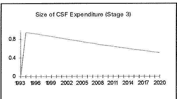
Percentage of GNP
Figure 5.2
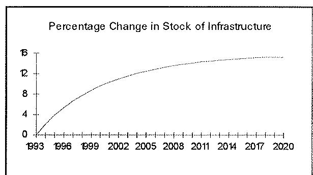
Percentage change relative to baseline
Since the CSF programmes are designed to promote cohesion in the EU periphery (i. e., convergence of real living standards), the primary effect of interest is their influence on real GDP. In Figure 5.3 we present the effects on real GDP at factor cost (GDPFC) for each of the first eight simulation stages. The graphs show the percentage increase over the non-CSF baseline.
The results of Stages 1 and 2 are very similar, with an impact of about 0.56% in GDP, peaking in 1997 and declining gradually over the rest of the simulation period to 0.45% by the year 2020. Of course, the implications for the domestic public borrowing requirement are very different, as will be illustrated below. The Stage 3 results are simply double of those of Stages 1 and 2, since we have assumed for illustrative proposes 1:1 domestic co-financing and the model is fairly lineal in its response to policy shocks.
The introduction of the factor productivity externalities in the N and T sectors (Stages 4 and 5, respectively) has different impacts on GDP. Whereas in the T sector, there is an intensification of the benefits beyond the Keynesian multiplier effects, the inflation proneness of the N sector erodes some demand effects from the year 2000. In effect, due to institutional and structural rigidities [see, e. g., OECD (1992)], cost pressures on the non-tradable sector are passed on the tradable sector and, through worsening in competitiveness, reducing its output. This highlights the need of structural reforms and a greater degree of competitiveness. When externalities are introduced into the output of the T sector (Stage 6), there is a dramatic increase in the impact of GDP, rising from the impact boost of 1.11% over the baseline level to around 3.06% by the year 2020.
As shown in Figure 5.3, Stage 7, when all the demand and externality effects are considered together, there are only slightly improved impacts over the Stage 6, rising to 3.33% by the year 2020. The need of gradually reducing the domestic borrowing requirements (Stage 8) attenuates these effects slightly, reducing them to 3.18% by the year 2020. Clearly, the infrastructure shock is not self-financing, even in the presence of 1:1 EU and domestic co-financing.
In Figure 5.4 we show for some key variables the difference between Stage 3 (Keynesian demand factors only), Stage 7 (full externalities, but not restriction placed on any deterioration of domestic public sector borrowing requirement) and Stage 8 (full externalities with a forced gradually reduction in public budget compared with no-shock baseline).
Figure 5.3: Infrastructure Shock: Effects on GDP att Constant Factor Prices
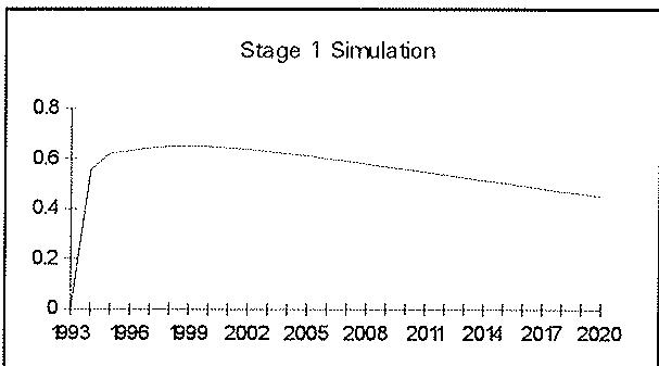
Percentage change relative to baseline
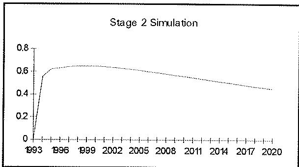
Percentage change relative to baseline
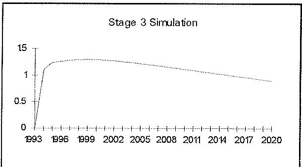
Percentage change relative to baseline
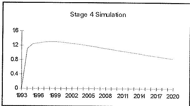
Percentage change relative to baseline
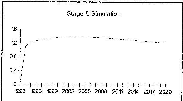
Percentage change relative to baseline
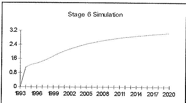
Percentage change relative to baseline
Percentage change relative to baseline
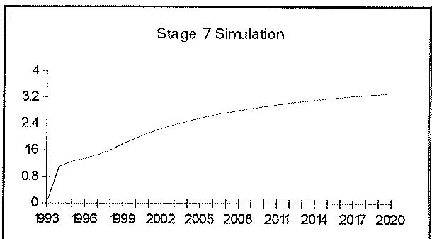
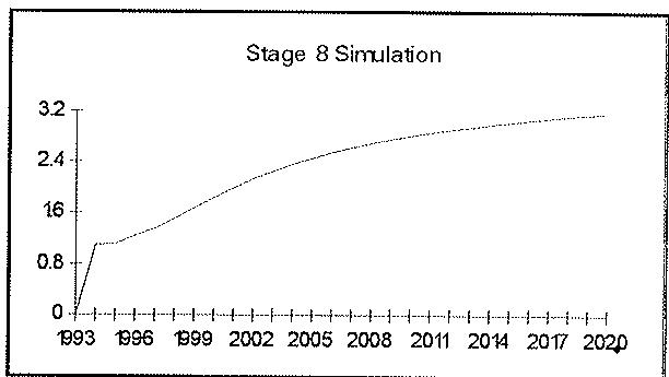
Percentage change relative to baseline
The effects on GDP at factor cost [graph (a)] have already been examined above. The effects on the domestic borrowing requirement are shown in graph (b). As can be seen, in the case of Stage 8 there is an obvious improvement, but while in Stage 3 there is a long-run deterioration of 0.08% points in GNP, in Stage 7 there is an improvement of 0.33% due to the rise in tax revenues. This is mirrored in the evolution of the debt/GNP ratio [graph (c)], which improves by 5.36 and 12.04 percentage points in Stage 7 and 8, respectively, while it deteriorates by 0.80% in Stage 3.
Regarding the balance of trade ratio [graph (d)], there is also a deterioration in Stage 3 (Keynesian) case by 0.51 percentage points of GNP, while the capacity-enhancing externality leads this to +0.49 and -0.36 percentage points in Stages 7 and 8. Finally, graph (e) shows the effects on unemployment. Even though in all three cases there is a negative initial effect, this improvement is wiped out in the long-run in Stages 7 and 8, while in Stage 3 there is a long-run reduction of 0.47%.
Figure 5.4: Stage 3,7 and 8 Infrastructure Shock Effects on Key Macro Variables. Percentage change relative to baseline
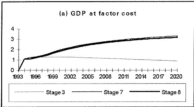
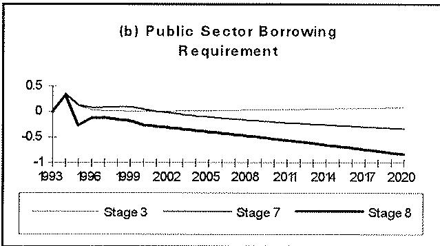
Change relative to baseline (% of GNP)
(c) National Debt / GNP Ratio Change relative to baseline (% of GNP)
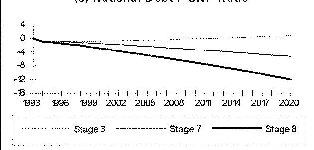
(d) Balance of Trade Change relative to baseline (% of GNP)
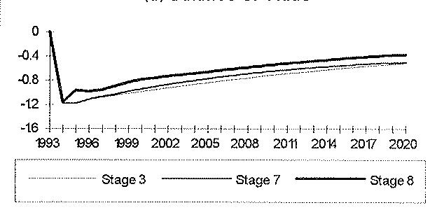
Change relative to baseline (% points)
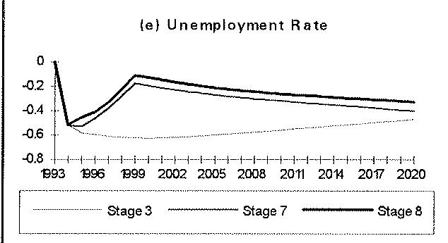
5.3 Ending the CSF: Hard or Soft Landing?
Although the current CSF covers the 1994-99 period, in the first eight stages above we assumed that the infrastructure shock (be it purely domestic, purely EU subvention or a 1:1 co-financing mixture) is continued ad infinitum and not ended in 1999. Stages 9 and 10 explore the consequences of an end in the EU aid subvention in 1999.
In Stage 9 we assume that, although the EU subvention ends, domestic public finance increases to close the financing gap. No restriction is placed on the public sector borrowing requirement, which will, in absence of EU aid, deteriorate compared with Stage 7 situation. In Stage 10 we simply cease the entire infrastructure shock and public spending reverts to the baseline non-shock state. Therefore, Stage 9 might be termed a "soft landing" and Stage 10 a "hard landing". Figure 5.5 shows, for Stages 7, 9 and 10, the effects on real GDP, on the public sector borrowing requirement, and on the public sector debt/GNP ratio.
From graph (a) we see that the substitution of domestic for EU financing has no effect on GDP at factor costs, being the Stages 7 and 9 GDP effects identical. However, there is a heavy price to pay in terms of increased borrowing and debt. In graph (b) we see that the borrowing requirement (expressed as a percentage of GNP) decreases in the year 2000 to 0.05 points in Stage 7, but it increases by 0.48 points in Stage 9, gradually reducing the gap between both Stages in the year 2020. From graph (c), the essential fall in the debt/GNP ratio in Stage 7 does not occur in Stage 9.
Regarding the comparison of Stage 7 and Stage 10, there is an abrupt decline in the boost of GDP from 1.80% in 1999 to 0.92% in 2000, mainly due to the sudden demand contraction that is assumed to take place entirely in the year 2000. There is a gradual improvement in the borrowing requirement, and the debt/GNP ratio stabilises at a fall of 1%.

Figure 5.5: Hard Landing or Soft Landing: Termination the Infrastructure Shock. (a) Effects on GDP
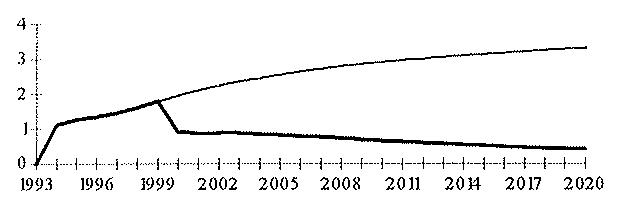
(b) Effects on Public Borrowing
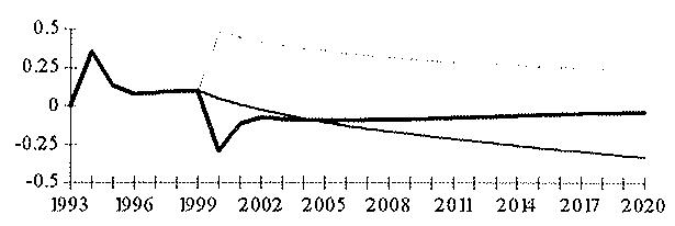

(c) Effects of Debt/GNP Ratio
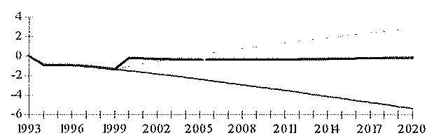
6. The CSF 1994-99 and its Effects on the Spanish Economy
In this section we present the results of the ex ante counter-factual experiments carried out to evaluate, in turn, the contribution to the growth of the Spanish economy from each of the three main component programmes of the CSF. The results are compared to a stylised projection (or baseline) for the economy to the year 2020.
Since the CSF proper starts in the year 1994, the pre-CSF baseline year is 1993. The effects of total expenditure under each of the three CSF programmes in the 1994-99 period are compared with the situation that would have prevailed in the complete absence of the CSF. Note that, due to our interest in the long-term impact on potential growth, the analysis is not ended in 1999, but is continued to the year 2020.
6.1 Physical Infrastructure
Table 6.1 shows the annual breakdown of the infrastructural programme. Using these data and the methodology outlined in the previous section we have quantified the effects of the CSF infrastructural programme in the Spanish economy.
| Table 6.1Spanish 1994-99 CSF funds on physical infrastructure (Bn. Pta) | |||||
| EU funds | Gov. sub. | Total pub | Priv. inv | Total | |
| 1994 | 238.7 | 148.5 | 387.2 | 0.0 | 387.2 |
| 1995 | 257.4 | 160.2 | 417.6 | 0.0 | 417.6 |
| 1996 | 277.6 | 172.7 | 450.3 | 0.0 | 450.3 |
| 1997 | 299.3 | 186.3 | 485.6 | 0.0 | 485.6 |
| 1998 | 322.8 | 200.9 | 523.7 | 0.0 | 523.7 |
| 1999 | 348.1 | 216.6 | 564.7 | 0.0 | 564.7 |
As mention above, we are primarily interested in the role of the CSF in promoting cohesion. Therefore, we will focus on the impacts on real GDP at factor cost. In Figure 6.1 we present two simulations showing the impact on that variable. The first one shows the Keynesian effects of the CSF shock (a Stage 3 simulation), excluding any positive externalities. The second one adds all three externality effects (a Stage 7 simulation) as described in section 5.2 above.
Figure 6.1: CSF Infrastructure Impact on GDP at factor cost. Percentage change over baseline. The Keynesian (Stage 3) impacts increase real GDP by 0.86% over the non-CSF baseline in 1994, rising gradually to 1.42% in 1999, and then steadily declining to 1.02% by the year 2020. The full impacts (Keynesian plus externalities: Stage 7) are initially the same in 1994, but have risen to 1.88% by 1999, reaching 3.68% in the year 2020.
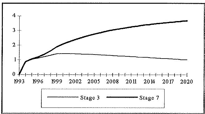
Table 6.2 summarises the CSF effects on some key macroeconomic variables besides GDP at factor cost.
| Table 6.2: CSF 1994-99 Infrastructural Effects | |||||||||
| 1994 | 1996 | 1999 | 2010 | 2020 | |||||
| Stage 3 | Stage 3 | Stage 7 | Stage 3 | Stage 7 | Stage 3 | Stage 7 | Stage 3 | Stage 7 | |
| Shock* | 0.74 | 0.83 | 0.83 | 0.97 | 0.97 | 0.74 | 0.74 | 0.57 | 0.57 |
| GDPfc** | 0.86 | 1.12 | 1.19 | 1.42 | 1.89 | 1.26 | 3.18 | 1.02 | 3.68 |
| Inflation** | 0.81 | 1.03 | 1.17 | 1.30 | 2.03 | 1.19 | 2.72 | 1.04 | 2.61 |
| Employment** | 0.72 | 0.95 | 0.75 | 1.22 | 0.43 | 1.10 | 0.62 | 0.90 | 0.76 |
| GBORR* | 0.18 | -0.05 | -0.01 | -0.09 | 0.00 | -0.13 | -0.37 | -0.10 | -0.55 |
| BPTR* | -0.91 | -1.01 | -1.01 | -1.15 | -1.11 | -0.80 | -0.73 | -0.57 | -0.55 |
| * Differences with respect to baseline** Percentual differences with respect to baselineNotes: Stage 3 computes the CSF full demand effects, while Stage 7 computes the latter and, in addition, the full supply effects. | |||||||||
As can be seen, the total public finance shock (EU subvention plus public domestic) makes up 0.74% of GNP in the initial year, gradually increasing to 0.97% by 1999, and then slowly declining to 0.57% by the year 2020. The decline is due to the fact that the financial injection is fixed from 1999 to its final value (i. e., Pta. 564.7bn), being only indexed to marginal price increases over the non-CSF price level.
Regarding inflation, in Stage 3 it rises from an initial increase of 0.81 percentage points over the baseline to a 1.30 in 1999, declining later to a 1.04 in 2020. However, in Stage 7, due to the inflationary pressures created by the N sector, there is an initial rise of 1.03 over the non-CSF baseline, progressively increasing to reach 2.61 in the year 2020.
Turning now to the effects on the labour market, after an initial increase of 0.72%, there is in both cases an increase in employment, but peaking in the Stage 3 simulation at 1.22% in 1999, and peaking in the Stage 7 at 0.75% in 1996.
Regarding the public sector borrowing requirement as a percentage of GNP (GBORR), there is an initial deterioration of 0.18% in that ratio, followed by a gradual improvement. Finally, the balance of trade/GNP ratio (BPTR) deteriorates by 0.91 percentage points of GNP in 1994, gradually improving over the simulation period.
6.2 Human Resources
Table 6.3 shows the annual breakdown of the human resources programme. Using these data and the methodology previously outlined we have also quantified the effects of the human resources CSF programme in the Spanish economy.
| Table 6.3Spanish 1994-99 CSF funds on human resources (Bn. Pta) | |||||
| EU funds | Gov. sub. | Total pub | Priv. inv | Total | |
| 1994 | 133.2 | 44.2 | 177.4 | 0.6 | 178.0 |
| 1995 | 143.6 | 47.7 | 191.3 | 0.7 | 191.9 |
| 1996 | 154.9 | 51.4 | 206.3 | 0.7 | 207.0 |
| 1997 | 167.0 | 55.4 | 222.4 | 0.8 | 223.2 |
| 1998 | 180.1 | 59.8 | 239.9 | 0.8 | 240.7 |
| 1999 | 194.2 | 64.5 | 258.7 | 0.9 | 259.6 |
Figure 6.2 presents the results of two simulations showing the impact of the human resources programme on real GDP: one shows the Keynesian (Stage 3) effects of the human resources on real GDP (excluding any positive externalities), and the other adds all three externality effects (a Stage 7 simulation) as described in section 5.2 above. Note that the Stage 7 simulations reported here have externalities associated with the improved shock of human capital that influence factor productivity in the T and N sectors and output in the T sector only.
Figure 6.2: CSF Human Resources Impact on GDP at factor cost. Percentage change over baseline. The Keynesian (Stage 3) impacts increase real GDP by 0.56% over the non-CSF baseline in 1994, rising gradually to 0.77% in 1999, and then steadily declining to 0.49% by the year 2020. The full impacts (Keynesian plus externalities: Stage 7) are initially the same in 1994, but have risen to 1.16% by 1999, and further to 2.58 in 2020.
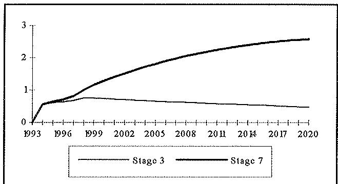
Table 6.4 summarises the CSF effects on some key macroeconomic variables in addition to GDP at factor cost. Note that the total public finance shock (EU subvention plus public domestic) constitutes 0.34% of GNP in the initial year, gradually increasing to 0.45% by 1999, and then slowly declining to 0.26% by the year 2020.
| Table 6.4: CSF 1994-99 Human Resources Effects | |||||||||
| 1994 | 1996 | 1999 | 2010 | 2020 | |||||
| Stage 3 | Stage 3 | Stage 7 | Stage 3 | Stage 7 | Stage 3 | Stage 7 | Stage 3 | Stage 7 | |
| Shock* | 0.34 | 0.38 | 0.38 | 0.95 | 0.45 | 0.34 | 0.34 | 0.26 | 0.26 |
| GDPfc** | 0.56 | 0.65 | 0.71 | 0.76 | 1.16 | 0.61 | 2.18 | 0.49 | 2.58 |
| Inflation** | 0.66 | 0.78 | 0.88 | 0.95 | 1.54 | 0.88 | 2.20 | 0.83 | 2.18 |
| Employm.** | 0.59 | 0.67 | 0.56 | 0.80 | 0.32 | 0.63 | 0.43 | 0.51 | 0.61 |
| GBORR* | 0.01 | -0.16 | -0.14 | -0.20 | -0.15 | -0.22 | -0.43 | -0.24 | -0.58 |
| BPTR* | 0.17 | 0.18 | 0.17 | 0.21 | 0.15 | 0.20 | 0.10 | 0.13 | 0.04 |
| * Differences with respect to baseline** Percentual differences with respect to baselineNotes: Stage 3 computes the CSF full demand effects, while Stage 7 computes the latter and, in addition, the full supply effects. | |||||||||
6.3 Aids to Production and Investment
Tables 6.5 to 6.7 show the annual breakdown of the aids to production and investment programme to the agricultural (A), non-traded (N) and traded (T) sectors, respectively. Using these data we have quantified the effects of the CSF-related expenditures on production aids in the Spanish economy.
| Table 6.5Spanish 1994-99 CSF funds on aids to A sector (Bn. Pta) | |||||
| EU funds | Gov. sub. | Total pub | Priv. inv | Total | |
| 1994 | 68.6 | 26.6 | 95.2 | 20.4 | 115.6 |
| 1995 | 74.0 | 28.7 | 4102.6 | 22.0 | 124.6 |
| 1996 | 79.8 | 30.9 | 110.7 | 23.7 | 134.4 |
| 1997 | 86.0 | 33.3 | 119.4 | 25.6 | 145.0 |
| 1998 | 92.8 | 35.9 | 128.7 | 27.6 | 156.3 |
| 1999 | 100.1 | 38.8 | 138.8 | 29.8 | 168.6 |
| Table 6.6Spanish 1994-99 CSF funds on aids to N sector (Bn. Pta) | |||||
| EU funds | Gov. sub. | Total pub | Priv. inv | Total | |
| 1994 | 61.2 | 28.0 | 89.1 | 106.7 | 195.8 |
| 1995 | 66.0 | 30.2 | 96.1 | 115.0 | 211.2 |
| 1996 | 71.1 | 32.5 | 103.7 | 124.0 | 227.7 |
| 1997 | 76.7 | 35.1 | 111.8 | 133.8 | 245.6 |
| 1998 | 82.7 | 37.8 | 120.6 | 144.2 | 264.8 |
| 1999 | 89.2 | 40.8 | 130.0 | 155.6 | 285.6 |
| Table 6.7Spanish 1994-99 CSF funds on aids to T sector (Bn. Pta) | |||||
| EU funds | Gov. sub. | Total pub | Priv. inv | Total | |
| 1994 | 52.3 | 21.9 | 74.3 | 81.4 | 155.6 |
| 1995 | 56.4 | 23.7 | 80.1 | 87.7 | 167.8 |
| 1996 | 60.9 | 25.5 | 86.4 | 94.6 | 181.0 |
| 1997 | 65.6 | 27.5 | 93.2 | 102.0 | 195.2 |
| 1998 | 70.8 | 29.7 | 100.5 | 110.0 | 210.5 |
| 1999 | 76.3 | 32.0 | 108.3 | 118.6 | 227.0 |
A key difference between this programme and the previous two is that there is a large private sector participation (17.7%, 54.5% and 53.3% in the A, N and T sectors, respectively). In Section 5.2 we have described how we handle this within HERMIN. Basically we assume that all such grants and aids to the private sector are contingent on private sector co-financing, being the co-financing ratios those implicit in Table 3.1.
In Figure 6.3 we present two simulations showing the impact of the production aids on real GDP. The first one shows the Keynesian (Stage 3) effects of the CSF shock (a Stage 3 simulation), excluding any positive externalities. The second one adds all three externality effects (a Stage 7 simulation) as described in section 5.2 above.
Figure 6.3: CSF Productions Aids Impact on GDP at factor cost.
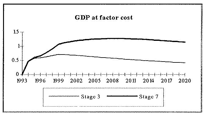
The Keynesian (Stage 3) impacts increase real GDP by 0.47% over the non-CSF baseline in 1994, rising gradually to 0.72% in 1999, and then steadily declining to 0.42% by the year 2020. The full impacts (Keynesian plus externalities: Stage 7) are initially the same in 1994, but have risen to 1.06% by 1999, and to 1.14 in 2020 after reaching 1.27% in the year 2008.
Table 6.8 summarises the CSF effects on some key macroeconomic variables besides GDP at factor cost. Note that the total public finance shock (EU subvention plus public domestic) is 0.49% of GNP in the initial year, gradually increasing to 0.65% by 1999, and then slowly declining to 0.34% by the year 2020.
| Table 6.8: CSF 1994-99 Production/Investment Aids Effects | |||||||||
| 1994 | 1996 | 1999 | 2010 | 2020 | |||||
| Stage 3 | Stage 3 | Stage 7 | Stage 3 | Stage 7 | Stage 3 | Stage 7 | Stage 3 | Stage 7 | |
| Shock* | 0.49 | 0.55 | 0.55 | 0.65 | 0.65 | 0.50 | 0.50 | 0.34 | 0.34 |
| GDPfc** | 0.47 | 0.59 | 0.66 | 0.72 | 1.06 | 0.55 | 1.26 | 0.42 | 1.14 |
| Inflation** | 0.44 | 0.54 | 0.60 | 0.65 | 0.98 | 0.51 | 1.19 | 0.42 | 1.17 |
| Employment** | 0.39 | 0.50 | 0.56 | 0.62 | 0.91 | 0.48 | 1.11 | 0.37 | 1.01 |
| GBORR* | 0.09 | -0.02 | -0.03 | 0.03 | -0.07 | 0.19 | -0.13 | 0.26 | -0.14 |
| BPTR* | -0.50 | -0.52 | -0.51 | -0.56 | -0.48 | -0.30 | -0.18 | -0.20 | -0.09 |
| * Differences with respect to baseline** Percentual differences with respect to baselineNotes: Stage 3 computes the CSF full demand effects, while Stage 7 computes the latter and, in addition, the full supply effects. | |||||||||
6.4 Total Spanish CSF 1994-99
We now combine the three shocks into a single simulation that examines the effect of the entire CSF 1994-99 on the Spanish economy.
As before, in order to quantify the role of the externality mechanisms, Figure 6.4 shows the results of two simulations showing the impact of the human resources programme on real GDP: one shows the Keynesian (Stage 3) effects of the total CSF on real GDP (excluding any positive externalities), and the other adds all three externality effects (a Stage 7 simulation) as described in section 5.2 above.
Figure 6.4-: CSF 1994-99: Total Impact on GDP at factor cost. Percentage change over baseline.
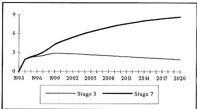
The Keynesian (Stage 3) impacts increase real GDP by 1.90% over the non-CSF baseline in 1994, rising gradually to 2.92% in 1999, and then steadily declining to 1.93% by the year 2020. The full impacts (Keynesian plus externalities: Stage 7) are initially the same in 1994, but have risen to 4.30% by 1999, reaching 8.65% in the year 2020.
Table 6.9 summarises the CSF effects on some key macroeconomic variables in addition to GDP at factor cost. Note that the total public finance shock (EU subvention plus public domestic) constitutes 1.55% of GNP in the initial year, gradually increasing to 2.03% by 1999, and then slowly declining to 1.21% by the year 2020.
| Table 6.9: CSF 1994-99: Total Effects | |||||||||
| 1994 | 1996 | 1999 | 2010 | 2020 | |||||
| Stage 3 | Stage 3 | Stage 7 | Stage 3 | Stage 7 | Stage 3 | Stage 7 | Stage 3 | Stage 7 | |
| Shock* | 1.55 | 1.73 | 1.73 | 2.03 | 2.03 | 1.56 | 1.56 | 1.21 | 1.21 |
| GDPfc** | 1.90 | 1.73 | 2.60 | 2.92 | 4.30 | 2.42 | 7.38 | 1.93 | 8.65 |
| Inflation** | 1.93 | 2.39 | 2.74 | 2.96 | 4.81 | 2.62 | 6.81 | 2.34 | 7.00 |
| Employment** | 1.71 | 2.14 | 1.89 | 2.64 | 1.78 | 2.22 | 2.68 | 1.78 | 3.32 |
| GBORR* | 0.29 | -0.23 | -0.18 | -0.26 | -0.27 | -0.16 | -1.15 | -0.09 | -1.71 |
| BPTR* | -1.19 | -1.31 | -1.29 | -1.44 | -1.32 | -0.91 | -0.67 | -0.62 | -0.47 |
| * Differences with respect to baseline** Percentual differences with respect to baselineNotes: Stage 3 computes the CSF full demand effects, while Stage 7 computes the latter and, in addition, the full supply effects. | |||||||||
7. A Comparison with the Irish and the Portuguese CSF 1994-99
All the regions in Ireland and Portugal are eligible for CSF funding under the Objective no. 1 of the Structural Funds while, in Spain, ten out of its seventeen Comunidades Autónomas are. Spain is the most favoured Member State of the EU concerning its share of total CSF funds originating in Brussels. However, given the size of its economy relative to the other two countries, the CSF expenditures represent considerably larger shocks to aggregate demand in the latter than in the former.
Once annualised, total CSF expenditures, including associated private investment, will amount, as percentages of national GDP, in 1994, to 3.7%, 6.4% and 1.6% in, respectively, Ireland, Portugal and Spain, as it is shown in the first column of table 7.1. The assumptions made about the rithm of CSF expenditure in every country combined with the increase of nominal GDP that each national HERMIN model produces makes the subsequent shocks to follow different courses afterwards.
For Ireland and Portugal, CSF expenditures are assumed to be constant in nominal terms while for Spain we adopted the criteria of the Spanish CSF whereby expenditure increases annually at about 10% in nominal terms. Of course, nominal GDP has a lower nominal increase per year so that the relative shock increases in Spain while it diminishes in Ireland and Portugal. In every case it was decided that, after 1999, when the current CSF will end, the shock is sustained unchanged under the same co-financing arrangements as before. The consequences of abruptly ending the CSF after 1999 have been explored in section 5.3 above.
| Table 7.1 CSF Growth Bonus in the EU Periphery | |||||||||
| CSF shock as % of GDP | GDPfc* - Stage 3 | GDPfc* - Stage 7 | |||||||
| 1994 | 1999 | 2020 | 1994 | 1999 | 2020 | 1994 | 1999 | 2020 | |
| Ireland | 3.7 | 5.4 | 3.1 | 1.7 | 2.7 | 1.8 | 1.7 | 3.8 | 4.6 |
| Portugal | 6.4 | 6.2 | 5.8 | 7.0 | 8.1 | 7.6 | 7.0 | 9.1 | 8.9 |
| Spain | 1.6 | 2.0 | 1.2 | 1.9 | 2.9 | 1.9 | 1.9 | 4.3 | 8.7 |
| * Percentual differences with respect to baseNotes: Stage 3 computes the CSF full demand effects while Stage 7 computes the latter and, in addition, the full supply effects.Sources: Bradley et al. (1994) and Table 6.9. | |||||||||
The growth consequences for each country are also shown in the table. After allowing for the full effects of the CSF in the whole period considered, the so-called Stage 7 explained in section 5.2, Ireland would have seen its GDP increased by 4.6% with respect to the no-CSF baseline with the externalities accounting for about two thirds of the total growth effect. In Portugal, the corresponding figures would be 8.9% with only 15% of the full growth effect due to externalities. Spain would receive a 8.7% growth bonus, 78% of which due to externalities.
These results are encouraging and show an interesting picture of the varying consequences of supra-national regional policies like the regional policy of the European Union towards its peripheral Member States. Each peripheral economy is different. It seems that, comparing the results of stages 3 (demand effects) and 7 (demand + supply effects), Portugal profits most from demand effects while Spain and Ireland get most of their respective growth bonuses from the supply effects.
The detailed discussion of these effects in the EU periphery is left however for next joint work by all the teams participating in this exercise.
8. Summary and Conclusions
8.1. The Major Effects of the CSF 1994-99
In Section 6.4 we saw that the total public finance shock (EU subvention plus public domestic) constitutes 1.55% of GNP in the initial year, gradually increasing to 2.03% by 1999 (the end of the CSF programme), and then slowly declining to 1.21% by the year 2020.
Our HERMIN-based CSF analysis stressed two possible effects: The traditional Keynesian impact (where the supply-side responses are assumed to be modest and limited to those induced by shifts in relative prices), and an augmented Keynesian response (where externalities associated with CSF programmes in infrastructure, human resources and aids to the private sector are incorporated).
As seen in Section 6.4, the Keynesian impacts of the CSF increase real GDP by 1.90% over the non-CSF baseline in 1994, rising gradually to 2.92% in 1999. On the other hand, the full impacts (Keynesian plus externalities) are initially the same in 1994, but have risen to 4.30% by 1999.
Moving the time horizon out to the very long term, if the public finance shock is maintained to its value in 1999, in the Keynesian case GDP steadily declines to 1.93% by the year 2020, while in the case of full impacts GDP rises further to 8.65 in 2020.
As we saw in Section 5.3, any form of "soft landing" is preferred to a "hard landing" after 1999, the terminal year of the current CSF. But such a "soft landing" would require the continuation of the infrastructural programme in form of gradually increased domestic funing to make up the difference after a reduction in the EU aid subvention. However, any such transition would bring pressure to bear on public finances that might prove unsustainable in the peripheral economies jeopardizing the cohesion objective.
8.2. Risks and Opportunities
Spain has an economy that has, since 1986 when it joined the EU, advanced considerably towards external liberalisation. It has also a developed economy that suffers however from severe structural desequilibria. Its growth pattern is reasonably in line with that of its major partners, when the desequilibria just mentioned permit. Although some of its Comunidades Autónomas are certainly backwarded relative to the average income standard of the EU, development, in the World Bank sense for example, is not the issue concerning the objectives of the Spanish CSF
Of course, the Spanish economy has to catch-up in real terms with the more advanced Members of the Union and may potentially suffer from increased economic integration. The real opportunity that CSF represent for Spain is, thus, the possibility to concentrate resources and efforts to upgrade the quality of the economic sectors, the skills of the work force and the infrastructure of the territories concerned.
At the stage of development where the Spanish economy founds itself, and facing the challenges it is facing, opportunities like the one mentioned before do not produce their beneficial effects for granted. Many other conditions, beyond the control of voluntarist policies, need to be met. Recall the discussion of section 4.3. We also showed the risk of loosing part of the crop if the favorable supply shock of the CSF are focused on the protected sector of the Spanish economy, the services sector. Productivity gains in this sector are translated to wages and these to prices more intensively than in the exposed sector, i.e. manufactures. This fuels inflation and competitiveness vis à vis the rest of the world worsens. This, paradoxically, punishes mostly the manufactures sector.
This risk is serious and its consequences go beyond the CSF success. Together with the imbalances in the labour market, the government accounts and the current account, it contributes to the unsustainability of any favorable shock the Spanish economy may receive.
Parrallel action, and intense, is thus needed on the internal liberalisation of the protected activities of the Spanish economy if the potencial benefits of the CSF are to be collected. On the other hand, given the challenges Spain faces in the internal market, the "new Europe", the post-Uruguay Round world, etc., the CSF interventions should have an increasingly strategic content.
8.3. Future Research
This exercise represents a considerable step forward for the Spanish team in charge of developing the HERMIN-Spain model. It is the first "acid test" of the model and to a large extent is preliminary. The model remains very simple, without finely tuned short or medium run properties and keeping exchange and interest rates parameterised. So, these are obvious areas for future development.
As for the CFS treatment itself, we pointed out before that only ten out of seventeen Spanish regions are receiving the CSF grants and thus we should be able to say something about the likely distribution of the growth bonus at least with in a simple North/South framework. This again waits and begs development in the very near future.
Concerning the team work and the joint exploitation of the models by all the national teams, much work could be done in order to ascertain the factors behind the differing results that the discussion of section 7 lets imagine. Indeed, given the strict comparability between the models, the different results should be attributed to the fact that the economies being analysed are different, provided the shocks are also equivalent. This is a complex exercise but a fascinating one given the challenges that European integration puts its periphery against and the prospects for an increased role of the Union's budgetary and regional policies as the economic integration crosses its "noble" stages [Krugman (1987)].
References
- Alcaide, J. (1993): "El Comportamiento Cíclico de la Economía Regional entre 1986 y 1992". Papeles de Economía Española, No. 55, pp. 2-30.
- Argimón, I., González-Páramo, J.M., Martín, M.J. and Roldán, J.M. (1993): "Productividad e Infraestructuras en la Economía Española". Documento de Trabajo No. 9313, Banco de España.
- Aschauer, D.A. (1989): "Is Public Expenditure Productive?". Journal of Monetary Economics, Vol. 23, pp. 177-200.
- Bajo-Rubio, O. y Sosvilla-Rivero, S. (1993): " Does Public Capital Affect Private Sector Performance? . An Analysis of the Spanish Case, 1964-1988". Economic Modelling, Vol. 10, pp. 179-185.
- Baldwin, R. (1989): "The Growth Effects of 1992". Economic Policy, No. 9.
- Bradley, J., Coimbra, R., Modesto, L., Neves, P.D. and O'Donnell, N. (1994): "The Effects of CSF 1994-99 on the Irish and Portuguese Economies: An Analysis based on the HERMIN Model". Technical Paper submitted to the European Commission.
- Bradley, J. and Wright, J. (1994): "HERMIN-I4: A Four-Sector Structural Model of the Republic of Ireland". Technical Paper submitted to the European Commission.
- Corujedo, I., García, E. and Martínez, J (1992): "Educación y Rentas. Una Aplicación a la Enseñanza Media en España: Una Nota". Investigaciones Económicas, Vol. 16, pp. 299-304.
- Cutanda, A. and Paricio, J. (1992): "Crecimiento económico y desigualdades regionales: el impacto de la infraestructura". Papeles de Economía Española, No. 51, pp. 83-101.
- De Hevia,, J. and Novales, A. (1992): "¿Es la Participación Activa Procíclica en España?", Documento de Trabajo 92-05. FEDEA.
- De Lamo, A.R. and Dolado, J.J. (1993): "Un modelo del Mercado de Trabajo y la Restricción de Oferta en la Economía Española". Investigaciones Económicas, Vol. 17, pp. 87-118.
- Draper, M. and J.A. Herce (1993): "Infraestructuras". Documento de Trabajo 93-07, FEDEA.
- Drèze, J.H. and Bean, C.R. (1990): "Europe's Unemployment Problem: Introduction and Synthesis". In Bean, C.R. and Drèze, J.H. (eds.) Europe's Unemployment Problem, Cambridge, Mass.: The MIT Press, pp. 1-65.
- Emerson, M., Aujean, M., Catinat, M., Goybet, P. and Jacquennin, A. (1988): The Economics of 1992: The EC Commission's Assessment of the Economic Effects of Completing the Internal Market. Oxford: Oxford University Press.
- Fernández, I. and Sebastián, M. (1991): "El Sector Exterior y la Incorporación de España a la CEE. Análisis a partir de Funciones de Exportaciones e Importaciones". In Molinas, C., Sebastián, M. and Zabalza, A. (eds.): La Economía Española: Una Perspectiva Macroeconómica, Barcelona: Antoni Bosch, pp. 209-303.
- García Delgado, J.L. et al. (1993): España, Economía. Madrid: Espasa Calpe.
- Herce, J.A. et al. (1994): "Evaluación del Marco de Apoyo Comunitario 1989-1993. Memoria Final", mimeo.
- Herce, J.A. and Sosvilla-Rivero, S. (1994a): "HERMIN-S3. A Three-Sector Structural Model of the Spanish Economy for the Analysis of Community Support Frameworks". Documento de Trabajo 94-01, FEDEA.
- Herce, J.A. and Sosvilla-Rivero, S. (1994b): "HERMIN Spain", fourth paper of an integrated set of six, entitled Modelling in the EU Periphery: The HERMIN Project, ESRI-UCP-FEDEA.
- INE (1993): Encuesta de Población Activa. Madrid: Instituto Nacional de Estadística.
- Krugman, P. (1987): "Economic Integration in Europe: Conceptual Issues". In Efficiency, Stability and Equity: A Strategy for the Evolution of the Economic System of the European Community (The Padoa-Schioppa Report). EC Commission, Doc. II/49/87.
- Krugman, P. (1991a): Geography and Trade. Cambridge, Mass.: The MIT Press.
- Krugman, P. (1991b): "Increasing Returns and Economic Geography". Journal of Political Economy, Vol.99, pp. 483-499.
- Krugman, P. and Venables, A.J. (1993): "Integration, Specialization and Adjustment". CEPR Discussion Paper, No. 886.
- Layard, R., Nickell, S. and Jackman, R. (1991): Unemployment: Macroeconomic Performance and the Labour Market. Oxford: Oxford University Press.
- Martin, P.J and Rogers, C.A. (1993a): "Trade Effects of Regional Aid". Paper presented at the CEPR/Yrjo Jahnsson Foundation Conference, May, Helsinki.
- Martin, P.J and Rogers, C.A. (1993b): "Industrial Location and Public Infrastructure", mimeo, Graduate Institute of International Studies, Geneva.
- Meade (1952): "External Economies and Diseconomies in a Competitive Situation". Economic Journal, Vol. 62, pp. 54-67.
- M.E.H. (1994): Plan de Desarrollo Regional 1994-1999. Regiones incluídas en el Objetivo No. 1 de los Fondos Estructurales Europeos. Tomo I. Madrid: Ministerio de Economía y Hacienda.
- Modesto, L. and Neves, P.D. (1993): "HERMIN-P4: A Four-Sector Structural Model of the Portuguese Economy". Technical Paper submitted to the European Commission.
- Molinas, C., Sebastián M. and Zabalza, A. (1991): La Economía Española: Una Perspectiva Macroeconómica. Barcelona: Antoni Bosch.
- Munnel, A. H. (1992): "Infrastructure Investment and Economic Growth". Journal of Economic Perspective, VOL. 6, pp. 189-198.
- OECD (1992): "Inflation Performance and Structural Rigidities". OECD Economics Surveys. Spain, pp. 54-76.
- OECD (1993): "Assessing the Effects of the Uruguay Round". Trade Policy Issues, No. 2.
- San Segundo, M. J. and Tohatia, L. (1993): "The Evaluation of Structural Funds Interventions in favour of Human Resources in Objective 1 Regions", mimeo.
- Sebastián, M. (1991): "Un análisis Estructural de las Exportaciones e Importaciones Españolas: Evaluación del Período 1989-1991 y Perspectivas a Medio Plazo". Información Comercial Española, No. 699, pp. 9-23.
- Sosvilla-Rivero, S. and Herce, J.A. (1994): "HERMIN-S4. A Four-Sector Structural Model of the Spanish Economy for the Analysis of Community Support Frameworks". Documento de Trabajo 94-08, FEDEA.
APPENDIX 1
THE SIMPC VERSION OF THE HERMIN-S4 FOUR-SECTOR MODEL OF SPAIN
(T) : Tradable sector - Industry (excluding energy) (N) : Non-tradable sector - Private services, building and construction, and energy (A) : Agriculture sector - Agriculture, forestry & fishing (G) : Public sector - Public administration, health and education
FEDEA: October 27, 1994
Eexogenous variables (excluded CSF) in the model are as follows:
| External variables | Financial var. | Public sector | Other | |||
| BPYPOTH | : | FXPD : | GEKO | GCNWR | GNDDR | DPARAT |
| GREVF | : | RL : | GNDFIX | GOSG | GTRSWR | DS |
| MP | : | GSUBR | GTYOR | IHGV | DSV | |
| OW | : | Demographic | GTER | GTYPR | LG | YAFSR |
| PMP | : | GREVO | GTYCR | WIGME | YFN | |
| POA | : | N1665 : | IGINF | GREVDIV | LTEMRT | |
| PWORLD | : | RGDI | IGVOTH | LAEMRT | ||
| PXA | : | UBENEFR | SCPR | LNAEMRT | ||
| ULCEC11 | : | PTROTH | PTRSWR | STATDIS | ||
| WIOME | ||||||
| ?The following parameters are estim | |
| ? | |
| PARAM AOT1 | -1.41355; |
| PARAM AOT2 | 0.11506; |
| PARAM AOT3 | 0.38865; |
| PARAM AOT4 | -0.11251; |
| PARAM AOT5 | -0.016647; |
| PARAM AOT6 | 0.75004; |
| PARAM APOT1 | 0.52776; |
| PARAM APOT2 | 0.59514; |
| PARAM AWT1 | -0.20985; |
| PARAM AWT2 | 0.98963; |
| PARAM AWT3 | -0.066273; |
| PARAM AWT4 | 0.69907; |
| PARAM AWT5 | -0.0049515; |
| PARAM AWT6 | -0.040250; |
| PARAM AON1 | 1788.19491; |
| PARAM AON2 | 0.46756; |
| PARAM AON3 | 119.48522; |
| PARAM APON1 | 0.91605; |
| PARAM AWN1 | -0.74192; |
| PARAM AWN2 | 1.14279; |
| PARAM AWN3 | -0.21977; |
| PARAM AWN4 | 1.69200; |
| PARAM AWN5 | -0.0072540; |
| PARAM AOA1 | 6.57849; |
| PARAM AOA2 | 0.014400; |
| PARAM ALA1 | 8.56141; |
| PARAM ALA2 | -0.048716; |
| PARAM AKA1 | -0.75803; |
| PARAM AKA2 | -0.014449; |
| PARAM AOG1 | 2.24529; |
| PARAM AOG2 | 0.70949; |
| PARAM AWG1 | 0.14447; |
| PARAM AWG2 | 0.95083; |
| PARAM APOG1 | -0.0071785; |
| PARAM APOG2 | 0.97792; |
| PARAM ALFPRM1 | 0.44019; |
| PARAM ALFPRM2 | -0.0014941; |
| PARAM ALFPRF1 | 0.11314; |
| PARAM ALFPRF2 | -0.0020655; |
| PARAM ALFPRF3 | 0.0050917; |
| PARAM ACONS1 | 0.20349; |
| PARAM ACONS2 | 0.94148; |
| PARAM ACONS3 | 0.031340; |
| PARAM ACONS4 | 0.011997; |
| PARAM AIHP1 | -2.45682; |
| PARAM AIHP2 | 0.86344; |
| PARAM AXA1 | -2.61047; |
| PARAM AXA2 | 0.070829; |
| PARAM AXT1 | 240.618; |
| PARAM AXT2 | 1.62885; |
| PARAM AXT3 | 1357.47; |
| PARAM AXT4 | -28.6228; |
| PARAM AXT5 | -476.197; |
| PARAM AXTUR1 | -1.93381; |
| PARAM AXTUR2 | 1.05101; |
| PARAM AXTUR3 | -1.15872; |
| PARAM AXNTUR1 | -0.40389; |
| PARAM AXNTUR2 | 0.90696; |
| PARAM APC1 | -0.040047; |
| PARAM APC2 | 0.91138; |
| PARAM APC3 | 0.80197; |
| PARAM APG1 | -0.066345; |
| PARAM APIH1 | -0.14148; |
| PARAM APIH2 | 0.98616; |
| PARAM APIH3 | 0.15095; |
| PARAM APIH4 | 0.033860; |
| PARAM APIG1 | -0.023513; |
| PARAM APIG2 | 0.83973; |
| PARAM APIT1 | -.024417; |
| PARAM APIT2 | .817956; |
| PARAM APIT3 | .170122; |
| PARAM APIN1 | .085609; |
| PARAM APIN2 | .593381; |
| PARAM APIN3 | .242393; |
| PARAM APIA1 | -.024399; |
| PARAM APIA2 | .817864; |
| PARAM APIA3 | .170198; |
| PARAM APXT1 | 0.16785; |
| PARAM APXT2 | 0.60489; |
| PARAM APXNTUR1 | -0.16805; |
| PARAM APXNTUR2 | 0.88820; |
| PARAM APXTUR1 | 0.065948; |
| PARAM APXTUR2 | 1.04780; |
| PARAM APGTE1 | 0.11615; |
| PARAM APGTE2 | 0.29593; |
| PARAM APGTE3 | 0.70184; |
| PARAM APGSUB1 | 0.054346; |
| PARAM APGSUB2 | 1.11636; |
| PARAM APYAFS1 | 0.25882; |
| PARAM APYAFS2 | 1.21574; |
| PARAM ADEP1 | -0.76850; |
| PARAM ADEP2 | 0.38962; |
| PARAM ADEP3 | 0.60621; |
| PARAM AYCU1 | -2.41208; |
| PARAM AYCU2 | 0.020343; |
| PARAM AYCU3 | 1.11213; |
| PARAM AT | 0.68820; |
| PARAM SIGT | 0.77498; |
| PARAM LAMLT | 0.037137; |
| PARAM LAMKT | -0.068719; |
| PARAM DELT | 0.97834; |
| PARAM AN | 1.17334; |
| PARAM SIGN | 0.51053; |
| PARAM LAMLN | 0.022571; |
| PARAM LAMKN | 0.027637; |
| PARAM DELN | 0.99242; |
? The following parameters are imposed, not estimated
? ALPHA is the weight in GBORR targeting rule
| PARAM ALPHA | 0.75 ; |
| PARAM ETATQI | 0.20 ; |
| PARAM ETATQH | 0.07 ; |
| PARAM ETATQPA | 0.10 ; |
| PARAM ETANQPA | 0.10 ; |
| PARAM ETATPI | 0.20 ; |
| PARAM ETATPH | 0.07 ; |
| PARAM ETANPI | 0.20 ; |
| PARAM ETANPH | 0.07 ; |
| PARAM OVERHD | 1.0 ; |
| PARAM OVERHDI | 0.10 ; |
| PARAM TMUP | 0.15 ; |
| PARAM FRACTED | 0.78 ; |
| PARAM TRATIO | 14 ; |
| END: |
END;
DOCUMENTOS DE TRABAJO
References
- 93-01: "¿Son las Cajas y los Bancos estratégicamente equivalentes?, Juan Coello.
References
- 93-03: "Indiciación salarial y empleo: un análisis desagregado para el caso español", María Draper.
References
- 93-04: "The productivity effects of fixed term employment contracts: are temporary workers less productive than permanent workers?", Juan F. Jimeno and Luis Toharia
References
- 93-05: "The determinants of labour mobility in Spain: who are the migrants?", Luis Albériko Gil and Juan F. Jimeno
References
- 93-06: "A survey of recent applied macroeconomic and modelling research on the Spanish economy", José A. Herce y Simón Sosvilla-Rivero.
References
- 93-07: "Infraestructuras", Maria Draper y José A. Herce.
References
- 93-08: "Los Servicios de transporte aéreo, marítimo y terrestre: estructura económica y regulación", Ginés de Rus.
References
- 93-09: "Situación actual, resultados y perspectivas del sector de las telecomunicaciones en España", Francisco Caballero.
References
- 93-10: "Estructura y Regulación del sistema sanitario Español", Guillem López i Casasnovas.
References
- 94-01: "HERMINS3, A three-sector structural model of the Spanish Economy for the analysis of Community Support Frameworks", José A. Herce y Simón Sosvilla-Rivero.
References
- 94-02: "El mercado de depósitos a la vista en España: Bancos vs Cajas de Ahorro", Juan Coello.
References
- 94-03: "An Econometric Analysis of Foreign Direct investment in Spain, 1964-89", Oscar Bajo-Rubio y Simón Sosvilla-Rivero.
References
- 94-04: "The management of redundancies in Spain: Econometric report", Juan F. Jimeno y Luis Toharia.
References
- 94-05: "Modelling international capital movements in the Spanish economy: A portfolio-balance approach". Oscar Bajo-Rubio y Simón Sosvilla-Rivero.
References
- 94-06: "Demanda de tráfico telefónico nacional en España 1985-1989: Un estudio econométrico con datos de panel provinciales", Teresa Garín.
References
- 94-07: "Demanda de tráfico telefónico internacional en España 1985-1989: Un estudio econométrico con datos de panel provinciales", Teresa Garín.
References
- 94-08: "HERMIN-S4, a four-sector structural model of the Spanish economy for the analysis of Community Support Frameworks", Simón Sosvilla-Rivero y José A. Herce.
References
- 94-09: "European railway comparisons and the future of RENFE", John Preston y Chris Nash
References
- 94-10: "The effects of the Community Support Framework 1994-99 on the Spanish economy: An analysis based on the HERMIN model", Jose A. Herce y Simón Sosvilla-Rivero.
Este texto se ha extraído automáticamente del documento original. Para citarlo o leerlo con su maquetación, descargue el PDF.
Descargar en PDF