A COST-BENEFIT ANALYSIS FRAMEWORK FOR SPANISH RAILWAY SERVICES
by
John Dodgson* and Mar Gonzalez Savignat**
Septiembre 1994
* University of Liverpool, England
** Universidad Carlos III de Madrid
Abstract
This Report is one of two which forms the research project on "Economic Aspects of Spanish Railways". The other report is by John Dodgson and Pablo Rodriguez Alvarez, and is titled "Profitability of the Different Services of RENFE".
The project was funded by the Banco de Espanà and FEDEA. We are extremely grateful to these organisations for their financial assistance, though we alone are responsible for the contents of this report.
We should like to thank Jose Hercé of FEDEA for facilitating the study. From RENFE, we particularly wish to thank Jesus Crepo and especially Rafael Almodóvar for all the information and assistance they provided for this study. Finally, we thank Paul Day for his research assistance at the University of Liverpool.
Contents
Introduction I The methodological framework II Travel time and its valuation III Accident costs and valuation IV Road traffic congestion V Environmental effects 1. Valuation of environmental effects 2. Localised air pollution 3. Global warming 4. Noise VI Cost-benefit analysis and RENFE's business units: a framework for appraisal VII A recommended research programme
INTRODUCTION
This Report is concerned with the application of social cost-benefit analysis techniques to Spanish railway services. Rail services receive substantial subsidies. A companion report to the present one (J.S. Dodgson and P. Rodriguez Alvarez "Profitability of the different services of RENFE") documents the financial position of RENFE's different business units. As Preston and Nash (1994, p.46) note in the report on their work which is complementary to our two reports, the level of subsidy on RENFE is high in relation to revenue in comparison with other European railways. It is important that value for money is secured in the payment of subsidy to railway services. Subsidy should only be paid if the social benefits which the rail service provides exceed the total costs of providing them. This means that the external benefits not captured in railway revenue should exceed the subsidies which Governments have to provide. As we indicate (Dodgson and Rodriguez Alvarez, 1994, p.55) it also means that all the costs of providing rail services, including infrastructure and capital costs as well as operating costs, must be included in the comparison of costs and benefits.
The appropriate way to measure the external benefits of rail services is through the use of social cost-benefit analysis. Carbajo and de Rus (1991) recommended that this technique be used to appraise investment in Spanish rail services, and de Rus and Inglada (1994) have recently applied the technique to the AVE route between Madrid and Sevilla. Preston and Nash (1994, pp. 46-47) recommend that social cost-benefit analysis be used for three distinct purposes in the Spanish railway industry:
• appraisal of new investments
• appraisal of the case for closing existing routes and concentrating traffic on the remaining parts of the system
• determining the optimal level of subsidy and the balance between rail service levels and fares in the main urban areas.
The present study has been concerned with the development of a framework for applying these techniques in Spain. Section I sets out the basic methodological framework for applying social cost-benefit analysis to rail services. It is based on the presentation in Dodgson (1984), and has been applied in Spain by de Rus and Inglada (1994). The Section identifies the main valuation issues involved in applying the technique to railways. These are to value travel time, accidents, road traffic congestion, and environmental effects such as noise and air pollution. These four issues are considered in Section II, III, IV and V of the report. The penultimate section of the report, Section VI, assesses how far these different benefits apply to RENFE's different business units and compares them with the existing estimates of the subsidies required. The final concluding Section outlines the main valuation and other exercises required to apply the techniques in Spain.
I.- THE METHODOLOGICAL FRAMEWORK
This Section of the report sets out the basic methodological framework for undertaking cost-benefit analyses of rail passenger services. Cost-benefit analysis is relevant in analysing rail services both because the benefits to rail users from a service might exceed the fare revenue they pay to the railway operator, and because there may be external benefits from the rail service.
Benefits to rail travellers can be measured using generalised cost and consumer surplus. This can be illustrated by considering the demand for transport services between one of the pairs of origin and destination served by the rail route.
Demand for travel is assumed to be a function of generalised cost per trip, g, where we suppose that;
\[\mathrm{g} = \mathrm{f} + \alpha_ {\mathrm{v}} \mathrm{t} _ {\mathrm{v}} + \alpha_ {\mathrm{w}} \mathrm{t} _ {\mathrm{w}}\tag{1}\]
and f = money cost (fare, operating costs, parking charges etc), and = in-vehicle and walking/waiting time, and = values of in-vehicle and walking/waiting time.
Figure 1 shows the position where bus is the only alternative transport mode, and bus and rail fares are equal. The difference between generalised cost per trip, g, and fare, f, gives the time cost per trip for each mode. By considering in turn the net benefits of the rail and the bus service we can derive the net benefit of the rail service as the benefit of having a rail service rather than an alternative bus service. The net benefits of rail and bus services are equal to the gross benefit under the demand curve, less resource (including time) costs incurred. Hence the net benefit of the rail service equals;
\[\mathrm{OacT} _ {\mathrm{r}} - \mathrm{fg} _ {\mathrm{r}} \mathrm{cd} - \mathrm{C} _ {\mathrm{r}} = \mathrm{g} _ {\mathrm{r}} \mathrm{ac} + \mathrm{OfdT} _ {\mathrm{r}} - \mathrm{C} _ {\mathrm{r}}\tag{2}\]
The net benefit of the alternative bus service is;
\[\mathrm{OaeT} _ {\mathrm{b}} - \mathrm{fg} _ {\mathrm{b}} \mathrm{ej} - \mathrm{C} _ {\mathrm{b}} = \mathrm{g} _ {\mathrm{b}} \mathrm{ae} + \mathrm{OfjT} _ {\mathrm{b}} - \mathrm{C} _ {\mathrm{b}}\tag{3}\]
£
Figure 1 User benefits of a rail service when the alternative mode of travel is bus
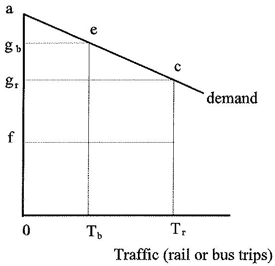
The area is equal to railway revenue, , and area is equal to additional bus revenue, . The term is the avoidable cost of the rail service and is the additional cost of the replacement bus service. and are not shown in Figure 1 since they are assumed not to be sensitive to small variations in the number of trips made because of the indivisibilities of operation.
The net benefit of retaining the rail service is then (2) minus (3);
\[\begin{array}{r l} & \left(\mathrm{g} _ {\mathrm{r}} \mathrm{ac} - \mathrm{g} _ {\mathrm{b}} \mathrm{ae}\right) + \left(\mathrm{R} _ {\mathrm{r}} - \mathrm{R} _ {\mathrm{b}}\right) - \mathrm{C} _ {\mathrm{r}} + \mathrm{C} _ {\mathrm{b}} \\ = & \mathrm{g} _ {\mathrm{r}} \mathrm{g} _ {\mathrm{b}} \mathrm{ec} + \left(\mathrm{R} _ {\mathrm{r}} - \mathrm{R} _ {\mathrm{b}}\right) - \mathrm{C} _ {\mathrm{r}} + \mathrm{C} _ {\mathrm{b}} \\ = & \mathrm{g} _ {\mathrm{r}} \mathrm{g} _ {\mathrm{b}} \mathrm{ec} + \left(\mathrm{R} _ {\mathrm{r}} - \mathbf {C} _ {\mathrm{r}}\right) - \left(\mathrm{R} _ {\mathrm{b}} - \mathbf {C} _ {\mathrm{b}}\right) \end{array}\tag{4}\]
This net benefit of retention is therefore equal to the increased time costs to rail travellers who would transfer to bus (area , or ), plus the loss to those who would no longer travel (area hec, or if the demand curve is assumed to be linear between points e and c), plus the loss of revenue incurred by public transport operators in the event of closure (area , or ), plus the costs of additional bus service provision ( ), minus the potential saving on the avoidable costs of the rail service ( ). We should also subtract from any additional benefits the extra bus provision would provide for existing or newly generated bus travellers. Using the same framework to analyse the case where rail and bus fares were different, it would be straightforward to show that net retention of the rail service would include the same items, except that the generalised cost losses to diverted and suppressed rail trips would incorporate changes in both time and money costs.
In practice, in the event of rail closure some former rail travellers will transfer to private cars, either as drivers or as passengers. Figure 2 illustrates the case where car is assumed to be the only alternative mode. The rail fare is denoted as and the behavioural car operating costs per trip, which must take account of car occupancy rates, as . The net benefit of car trips is equal to the gross benefit under the demand curve, less time and resource costs. If resource and behavioural car costs were equal then from Figure 2 the net benefits of car trips would be:
\[\mathrm{OamT} _ {\mathrm{c}} - \mathrm{f} _ {\mathrm{c}} \mathrm{g} _ {\mathrm{c}} \mathrm{mp} - \mathrm{Of} _ {\mathrm{c}} \mathrm{pT} _ {\mathrm{c}} = \mathrm{g} _ {\mathrm{c}} \mathrm{am}\tag{4}\]
Subtracting (4) from (2) we then find the net benefit of rail retention as equal to:
\[\left(\mathrm{g} _ {\mathrm{r}} \mathrm{ac} - \mathrm{g} _ {\mathrm{c}} \mathrm{am}\right) + \mathrm{R} _ {\mathrm{r}} - \mathrm{C} _ {\mathrm{r}}\tag{5}\]
This net benefit of retention is equal to increased generalised costs to rail travellers who would transfer to car (area , or ), plus the loss to those who would no longer travel (area nmc, or ), plus the rail revenue lost ( ), minus the potential saving on the avoidable costs of the rail service ( ). In addition, we should add to the benefits of the rail service any increases in the costs of highway provision (both capital and maintenance) which were regarded as essential in the event of rail closure, less any additional benefits this provision would create for existing or newly-generated highway users.
Figure 2 User benefits of a rail service when the alternative model of travel is car
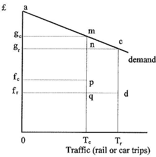
If a rail service is no longer operated some former rail travellers will travel by bus, some by car, a few by bicycle, foot or taxi, and some will not travel or will make a trip to a different destination. The methodology we have outlined can be used to determine generalised cost changes for all these groups. Where trips are no longer made, the appropriate treatment is to view the former traveller as not valuing this trip as highly as the minimum generalised cost by the alternative modes which are available for him to make that particular journey.
The second major justification for cost-benefit analysis of rail services is the existence of external benefits of rail service provision, in the form of reduced road accidents, reduced highway congestion, and reduced environmental effects.
Where some former rail travellers divert into cars which travel on already congested roads, there will be costs to existing road users. These can be measured by taking the predictions of former rail users diverting to car, assigning the resulting increase in car trips to the road network parallel to the railway, and then combining this information and data on existing traffic levels on these routes with speed/flow curve and operating cost formulae to calculate the increase in operating and time costs to existing traffic. An iteration then needs to be performed to allow for the effects of these increased operating and time costs in diverting some of the existing road traffic onto other parts of the network, or suppressing it altogether. The predicted increases in road vehicle flows can also be used in conjunction with accident rate data to predict increased numbers of road accidents. Allowance must also be made for any expected reduction in rail casualties, both to passengers and to railway employees, if the rail service were no longer operated.
Rail services might also provide environmental benefits if they reduce the amount of noise, air pollution and other environmental externalities associated with other transport modes. An issue of current concern is the global warming effects of emissions from the transport sector, particularly carbon dioxide from burning fossil fuels.
In the next four Sections of the report we review the main measurement and valuation issues which would be involved in applying social cost-benefit analysis to Spanish railways, under the headings of Travel time and its valuation (II), Accident costs and valuation (III), Road traffic congestion (IV), and Environmental effects (V).
II.- TRAVEL TIME AND ITS VALUATION
There are two main issues here: (1) measuring the time savings created by rail services (2) valuing travel time in monetary terms. If rail services are slower than other modes, then there will be no time benefits from their retention. In some cases Spanish rail services will be slower than car and slower than the coach services using the road network. Table 1 shows times on some long-distance routes.
Table 1: Comparative travel times and fares by coach and train, selected corridors
| COACH | RENFE | |||
| Time(hours) | Fare(ptas) | Time(hours) | Fare(ptas) | |
| Madrid-Valencia | 4:30 | 2,540 | 3.55(IC) | 2,900 |
| Madrid-Bilbao | 5:00 | 2,950 | 6:30(T) | 3,900 |
| 8:55(S) | 3,900 | |||
| 6:00(C) | 3,800 | |||
| Madrid-Vigo | 8:30 | 3,075 | 10:25(S) | 4,800 |
| 7:55(T) | 6,800 | |||
| Madrid-Barcelona | 8:00 | 2,660 | 8:15(IC) | 5,400 |
| 7:15 | 3,415 | 6:45(T) | 4,500 | |
| 8:50(S) | 4,500 | |||
T: talgo; S: star trains (overnight); IC: intercity Note: All the fares in the table are "second class". Star trains are overnight trains, but the fares in the table exclude the supplement of 1,800 pts. for a sleeping berth.
Preston and Nash (1994, pp. 6, 10) note that in general Spanish rail services are slow in relation to those of other European countries. Consequently travel time benefits of rail services are most likely to be relevant for high-speed services, and for commuter services in urban areas when road traffic is affected by congestion.
When we turn to the issue of valuation of travel time, there are two major types of travel time to consider. These are travel in the course of work, and travel in leisure time. The latter category of leisure, or non-working time, generally includes travel to and from work, i.e. commuting time. Travel in working time is relatively straightforward to value by means of reference to the wage costs incurred by employers. Leisure, or non-working, time is much more difficult to value because there is no market for leisure time, and hence no market value for it. Early work in Britain mainly used data from actual travellers facing a trade-off between time and money to derive their valuations of marginal savings in travel time. This approach is known as the revealed preference (RP) approach. In the 1980s the UK Department of Transport commissioned a major series of studies on travel time (MVA, et al, 1987). Although some of the studies used revealed preference methods, others used stated preference (SP) methods, and some used both.
While revealed preference methods require data from people facing actual trade-offs (for example, a rail traveller who could alternatively travel by a slower but cheaper bus service - and hence is in effect paying money to save time), stated preference methods present individuals with hypothetical trade-off choices and ask them to state their preferences. Because of this, a very much wider range of situations can be considered, but the participants do not have to consume their choices (i.e. reveal their preferences through actual travel behaviour).
Seven major surveys were carried out in the 1980s in Britain, in different parts of the country, and looking at different types of travel (urban buses, inter-urban car, urban car, long distance rail and coach, commuter rail and coach). Where RP and SP methods were used in the same study, they appeared to yield similar results, hence increasing confidence in the SP approach. Values of time were derived for a variety of situations, and as a consequence the Department of Transport modified the values of time recommended for project appraisal: in particular the value of in-vehicle non-working time was increased from 25 per cent to 43 per cent of average hourly earnings.
We can gain some ideas of time valuation in Spain by considering the labour costs inquiry published in 1991 by the National Institute of Statistics. This gives an average annual cost per employee in 1988 of 2,144,100 pts. This is made up of: wages, 1.592 million pts. (73.5 per cent); national insurance, 0.485 million pts. (22.4 per cent); and social payments, 0.034 million pts. (1.6 per cent). Applying the increase in the wage index for Spain from 1988 to 1992, and a figure of annual hours worked per person per year of 1,769 hours (Anuario Estadístico de Espana, 1992) gives an average cost per employee to the employer of 1,637 pts. an hour or 27.3 pts. a minute.
If no data were available on the form of employment of employees travelling in working time on a particular rail service, then this figure gives an appropriate indicator of working time travel valuations. The theory of travel time value suggests that leisure time will be valued at less than working time. If we apply the British result that non-working time is valued at 43 per cent of the wage rate (as opposed to wage cost), we derive an estimate of non-working time in Spain as
\[(1, 6 3 7 \times 0. 7 3 5 \times 0. 4 3) = 5 1 7 \text { pts an hour }\]
or 8.6 pts. a minute.
This figure can only give a broad indication of leisure time travel values in Spain, and detailed work is needed to estimate travel time values under different circumstances (eg rail travellers, bus travellers, car travellers, short-distance travellers, long-distance travellers). Ana Matas (1990) estimated travel time values in Spain using a demand function with a probit model. The value of time at 1988 prices obtained varied between 169 pts. an hour for non-qualified people to 644 pts. an hour for qualified travellers, with an average value across the sample of 242 pts. an hour, or 4 pts. a minute. Matas points out that differences in time values will arise partly because of differences in the way time is spent: waiting time savings are valued three times more highly than in-vehicle time savings, though walking time is valued similarly to in-vehicle time.
Hunt (1992) used a logit model to analyse in-vehicle travel time in Barcelona. Data were collected on route choice decisions made by car travellers in the city, in order to value the benefits of a new expressway. This study derived average values for in-vehicle time at 1989 prices of 46.4 pts. per vehicle-minute, or 30.1 pts. per person-minute. These figures are high in relation to Matas' estimates and to our own estimate of 8.6 pts per person-minute, even though Hunt's estimates relate specifically to car users.
de Rus and Inglada (1994) used values of time savings from MOPT (1991). At 1993 values these were:
| Per hours (pts) | Per minute (pts) | |
| Coach | 758 | 12.6 |
| Train | 1633 | 27.2 |
| Bus | 408 | 6.8 |
| Aeroplane | 3208 | 53.5 |
Time savings form the major component of the external benefits of AVE evaluated by de Rus and Inglada. de Rus and Inglada also recommend a major effort of research in valuing travel time for different types of travellers and different modes in Spain.
III.- ACCIDENT COSTS AND VALUATION
Where accident rates are higher for road transport than rail transport, provision of rail services may provide benefits in the form of reduced road accident costs. UIC statistics show the accident death rate per hundred million passenger-kms plus tonne-kms to be 2.1 for rail in Spain, and 21.1 for road transport in Spain. In 1991 there were 6,797 road fatalities and 155,247 injuries. Railway casualties can vary from year to year, but the average number of fatalities on RENFE between 1980 and 1991 was 35.5 per year. Our own calculations yield figures of death rates on RENFE of 2.4 per thousand million passenger-km, and on Spanish roads of 28 per thousand million passenger-km. The equivalent accident rates for RENFE and roads are 3.5 and 650 respectively per thousand million passenger-km. This means that the road death rate per unit of traffic is 11.9 times greater than the rail death rate, while the road injury rate per unit of traffic is 186 times greater than the rail injury rate.
A crucial consideration in any cost-benefit evaluation of rail services is how the number of accidents would change if the services were withdrawn. This requires us to predict not only the amount of traffic that will transfer to other modes, but also the question of whether accident rates along a particular length of road will change when the traffic volume changes.
The second important consideration is how to value accident costs. Some costs can be valued because they relate to financial costs such as physical damage to vehicles. More difficult are the costs of personal injury, and particularly loss of life. A common but incorrect method applied to value loss of life is the loss of output, or "human capital" approach. The gross output method discounts the accident victim's expected future earnings over the rest of their expected life:
The net output method subtracts expected future consumption, , from income.
However neither method is correct, since neither are consistent with the welfare economics foundations of cost-benefit analysis. What is relevant is not the value of any individual's life, but the valuations of small changes in risk of all those affected by potential changes in transport accident risk. These small changes in risk should be valued by reference to willingness to pay. When the valuations are added up over all the risks which add to the risk that one life will be lost, they provide a valuation of the concept of "a statistical life". There are two main ways to value this, the revealed preference approach, and the survey (or stated preference) approach.
The main source of revealed preference values of risk is the labour market. This is because wage differentials between jobs will reflect, amongst many other factors, an allowance for the risk of death in the different jobs. Marin and Psacharopolous (1982) used a regression model to investigate the extent to which wages in the UK labour market are influenced by occupational risk of death. Annual earnings were regressed on years of schooling and years of labour market experience (both of which reflect human capital factors), on unionisation variables, on variables reflecting occupational desirability, and on general and accident risk in the workers' occupation. General risk is the overall risk of death in a particular job, and includes risk of death from occupationally-induced illnesses such as silicosis and asbestosis, while accident risk is the risk of death in an accident while at work. Accident risk, which Marin and Psacharopolous argue is more likely to be correctly perceived than general risk, was found to be statistically significant. Multiplying the increased earnings associated with an increased risk of death in a year by the inverse of the increased probability of death yields a value of life, in the sense of the labour market's evaluation of a "statistical death". This is the sum of a large number of individuals' willingness to accept monetary compensation for a small increase in their own risk of death where the total probability of increased loss of life sums to one; that is, it is not the valuation of the life of a single, known, individual. Though valuations varied between different types of worker, Marin and Psacharopolous derived an overall value of around £1.9 million when converted to 1988 price levels.
In the UK the stated preference, or survey approach, has been pioneered by Jones-Lee. The most detailed study was one commissioned by the Department of Transport and carried out by National Opinion Polls (Jones-Lee, et al, 1985). A nationally representative personal survey yielded over one thousand responses to a complex set of questions on attitudes to, and valuations of, risk. In particular respondents were asked how much they would pay to travel on coach services with different degrees of risk, and how much they would pay for safety features for their cars which were associated with different degrees of risk. Various values for a "statistical life" were then derived. A major feature of the results was that the values were broadly consistent with those derived by Marin and Psacharopolous in their labour market study. As Jones-Lee et al note "The fact that two studies concerned with different types of risk, using radically different methods and completely different samples produce such similar estimates is ... very powerful evidence in favour of the credibility of these estimates" (Jones-Lee, et al., 1985, p. 71).
The results of these willingness-to-pay studies were eventually accepted by the UK Department of Transport, and the values of the costs of fatal accidents were revised upwards as willingness-to-pay values replaced gross output methods. Recent work (O'Reilly, et.al., 1994) has extended this approach to value non-fatal injuries in road accidents.
Spanish values for casualties are based on a percentage of per capital average income. The values recommended by MOPT in 1987 pts. are:
Fatal casualty 15,730,000pts
Serious injury 1,580,000 pts
These can be compared with UK willingness to pay values, which are at 1992 prices. To do this we adjusted the Spanish values to Spanish 1992 prices using the change in the RPI in Spain between 1987 and 1992. The UK values were adjusted to allow for differences in per capital GDP between Spain and the UK in 1992 (GDP per capita in Spain was 82.8 per cent of that in the UK). The revised UK values were then converted to ptas. by adjusting by the OECD figure for purchasing power parity for GDP between Spain and the UK in 1992 (176.38). The resulting comparison is shown in Table 2, and shows how the MOPT figures are very much lower than those based on this willingness-to-pay comparison. This suggests that road accident costs may be seriously undervalued in Spain. However, research work on willingness-to-pay measures for Spanish travellers is needed to derive correct values for Spain.
Table 2 : Valuation of fatal and serious casualties 1992
| UK willingness to pay value in UK £s | UK willingness to pay value converted to pts. and adjusting for real income differences | MOPT values adjusted to 1992 prices | |
| Fatal | £634,600 | 92.5 m pts | 21.1 m. pts |
| Serious | £71,100 | 10.4 m pts | 2.1 m. pts |
IV.- ROAD TRAFFIC CONGESTION
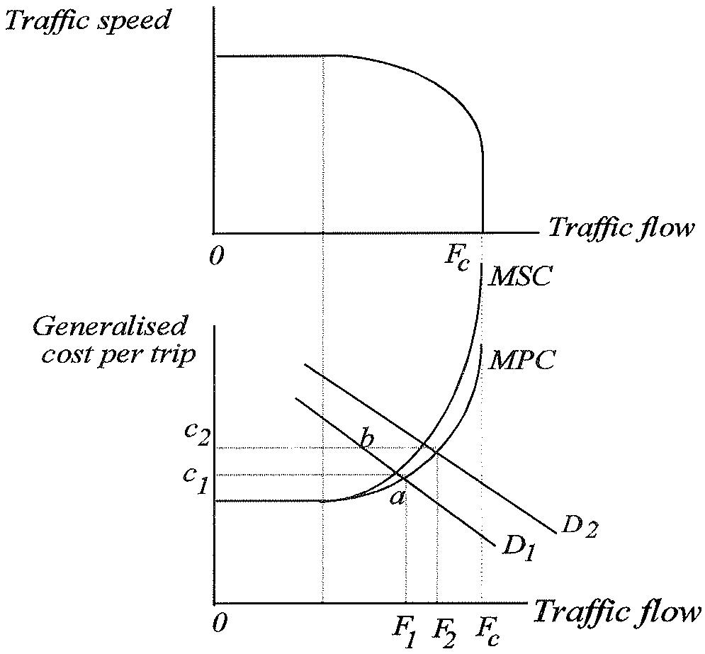
As we indicated in Section I, provision of rail transport services may ease road traffic congestion. Consider Figure 3, where traffic flow along a stretch of road is shown along the horizontal axis. The top part of the diagram shows the speed-flow curve for the road, and the bottom part shows generalised cost per car trip, and demand for travel. At low traffic volumes average cost per trip, i.e. marginal private cost (MPC), is equal to marginal social cost (MSC), since there is no traffic congestion where the speed-flow curve is horizontal. Then as traffic volumes increase this causes the speed of traffic to fall, and speed falls as traffic rises until the physical capacity of the road, , is reached. Once congestion occurs, each additional vehicle slows down all other vehicles, so the marginal social cost exceeds marginal private cost. In the normal situation where there is no congestion charging system for roads, the equilibrium traffic flow will be at , where the demand curve cuts the MPC curve. The resulting generalised cost per trip is .
Suppose that shows road demand when a parallel rail service is in operation. Now suppose the rail service were not in operation, so that road demand shifted out to . This would then increase generalised cost per trip to , and impose additional time and operating costs on existing road users equal to the area ba. In order to calculate such additional external benefits of rail service provision, we need information on:
(1) the speed-flow and other engineering relationships (such as junction delay formulae) for the congested roads. One approach is to use values from the US Transportation Research Board (1985), though values derived specifically for Spanish road conditions would be more satisfactory.
(2) operating cost formulae which show the relationship between speed and operating costs per vehicle-km for the congested roads. The relevant operating costs are the costs of fuel, lubricants, tyres, and those parts of vehicle maintenance and depreciation that vary with use. MOPT (1992) refers to a study carried out for the MOPU in 1977 for three types of vehicles, car, lorries and buses. These relate the various components of operating costs to traffic speed.
(3) time values for the existing users of the congested roads, since time forms an important component of generalised cost (see Section II above). Travel time is obviously related inversely to traffic speed.
(4) predictions of the numbers of rail users who will switch to car if the rail service is withdrawn.
When cost-benefit analysis is being used to assess the benefits of different levels of subsidy for urban rail services, when these subsidies will be used to lower rail fares and/or improve service levels (see Dodgson, 1986; Glaister, 1987), item (4) above needs to be replaced by (4'), the cross-elasticities of demand between car travel and rail fare and rail service quality. Of course if these cross-elasticities are zero, there are no congestion-reduction benefits in subsidising rail.
Cross-elasticity values can be derived by considering their relationship with own-price or own-service elasticities. For example, if an urban commuter rail service has an own-fare elasticity of -0.20, a one per cent reduction in rail fare will lead to a 0.2 per cent increase in rail demand. Some of this increase should come about through diversion from private cars, and this part of the increase can be related to the original level of private car traffic. It can be shown (Dodgson, 1986) that the own-price and cross-price elasticities are related to each other, both via this proportion and via the relative levels of users (or modal shares) of the two methods of transport. Thus:
\[\mathrm{e} _ {\mathrm{af}} = - \mathrm{e} _ {\mathrm{f}}. \delta_ {\mathrm{f}}. (\mathrm{m} _ {\mathrm{r}} / \mathrm{m} _ {\mathrm{a}})\]
where cross-elasticity of automobile trips with respect to rail fare
rail own-fare elasticity of demand
proportion of any increase in rail travel as a result of a rail fare change that is diverted from automobile trips.
= modal share of the rail mode (or level of rail traffic)
= modal share of the automobile mode (or level of automobile traffic).
Similarly for rail service level cross-elasticities
\[\mathrm{e} _ {\mathrm{as}} = - \mathrm{e} _ {\mathrm{s}}. \delta_ {\mathrm{s}} \left(\mathrm{m} _ {\mathrm{r}} / \mathrm{m} _ {\mathrm{a}}\right)\]
where cross-elasticity of automobile trips with respect to rail service elasticity
= rail own-service elasticity of demand
proportion of any increase in rail travel as a result of a rail service level increase that is diverted from automobile trips.
These formulae show that, other things equal, the cross-elasticities will be lower, the lower is the initial share of rail transport in the market.
For illustrative purposes, we have applied these formulae for Barcelona and Madrid, Economic literature on demand elasticities in other countries suggests a value for own-fare elasticity for rail commuter services of around -0.2. Table 3 shows passenger-km data for commuter rail and private car in Madrid and Barcelona.
Table 3: Mode shares in Madrid and Barcelona, million pas.-km
| Commuter rail | Private car | $m_r/m_a$ | |
| Madrid | 2.651 | 16.000 | 0.17 |
| Barcelona | 1.717 | 28.364 | 0.06 |
Evidence on the diversion factors, which must lie between zero and one, is not available, so we take a value of 0.25 for illustrative purposes. This yields fare cross-elasticity estimates as follows
\[\begin{array}{l l l l} \text {Madrid} & e _ {a f} & = & 0. 0 0 8 5 \\ \text {Barcelona} & e _ {a f} & = & 0. 0 0 3 0 \end{array}\]
The first of these illustrative figures indicates that a ten per cent fall in commuter rail fares in Madrid would lead to a 0.085 per cent (or less than one tenth of one per cent) fall in car traffic on Madrid's road network. This number is small, but it is a small percentage change in a very large volume of traffic, so the effects on road congestion may not be insignificant.
V.- ENVIRONMENTAL EFFECTS
1. Valuation of environmental effects
Environmental effects have proved to be more difficult to evaluate in monetary terms than either time or accidents. In part this stems from the difficulty of measuring many environmental effects in physical units as a prelude to valuing them. Two main approaches have been used to value environmental effects:
• the hedonic house price approach
• contingent valuation methods
Hedonic prices
The value of a piece of land is related to the benefits derived from that land. The house price is the best example of this. If different locations have varied environmental attributes, such variations will result in differences in property values. The way to infer the monetary values of the different attributes is through the use of multiple regression analysis relationships between house prices and environmental quality levels, in order to discover how much people are willing to pay for an improvement in environmental quality. The regression coefficient on the environment variables could be interpreted as the capitalization of differences in these variables. However, differences in residential property prices can be attributed to many variables. Therefore, in order to pick up the effects of environmental quality on the price of housing, all significant variables must be identified, since bias can result from the exclusion of relevant variables.
The hedonic house price approach has been used in the monetary evaluation of noise and air pollution. Earlier studies of the effects of airport and road traffic noise on property values were surveyed by Nelson (1980, 1982). Pearce and Markandya (1989) have provided an excellent more recent survey. The main conclusions are as follows:
• The impact of traffic noise on house prices Results are presented in terms of the impact of a one unit change in as a percentage change in house prices. is the Equivalent Continuous Sound Level, the level of constant sound which would have the same sound energy over a given period as the measured fluctuating sound under consideration. Studies, mainly from the US, show percentage changes in house prices varying between 0.08 and 1.26 per cent. The average effect of an increase in traffic noise of one decibel is a reduction in house prices of about one half of one per cent.
The impact of aircraft noise on house prices Results are presented in terms of the impact of a one unit change in NEF or NNI as a percentage change in house prices. NEF and NNI are measures of aircraft noise related to human hearing and discomfort. Pearce and Markandya (1989, p.29) conclude that the results are fairly consistent, and suggest that a unit increase in NEF would reduce property values by about 0.7 per cent, while a unit increase in NNI would reduce them by about 0.5 per cent.
The impact of air pollution on property values Results are presented in terms of elasticities between changes in air pollution and property values. All the results are for the USA, and show elasticity estimates for sulphation, particulates, oxidants and dustfall. One major problem with these studies is that it is not possible to separate out the effects of different pollutants.
Contingent valuation methods
With Contingent Valuation methods individuals are surveyed in order to elicit their monetary evaluations of environmental effects. They may be asked what they are willing to pay to achieve a certain environmental benefit, or what they are prepared to accept to have to put up with a particular environmental cost. The surveys may be conducted through the use of questionnaires, or through experiments in laboratory conditions.
As the Contingent Valuation method is a form of Stated Preference technique, it suffers from the problem that individuals are not forced to consume their choices, so that their real-world valuations in terms of willingness-to-pay (WTP) or willingness-to-accept (WTA) might be different. There may also be problems in conveying to respondents the particular environmental effect under consideration, such as a particular level of traffic noise, or a particular type of air pollution. Sometimes, respondents may believe that their answer may influence the monetary payment they may receive: consequently, they have an incentive to bargain, for example claiming that no amount of compensation may recompense them for putting up with an increase in the traffic noise outside their house. The initial sum suggested as compensation for an environmental change might also influence the eventual outcome of the bidding process. People may also be influenced by the form in which payment is to be made, perhaps preferring entrance fees to taxes, or road congestion charges to increases in local taxation. There may be biases as a result of the way information about the hypothetical changes are communicated to the respondents by the surveyor. Many studies suggest that there is a divergence between WTP and WTA, so that individuals would not be prepared to pay in practice as much as they claim they would require in compensation.
These and other potential sources of bias are discussed by Pearce and Markandya (1989). Contingent Valuation methods have been used in the transport sector in the UK, but so far it has proved difficult to derive consistent valuations of even the more common environmental costs of transport.
Environmental effects and health
Where specific environmental effects have a measurable effect on health, it is in principle possible to measure the effects of changes in the environmental effect on mortality and morbidity, and then value these effects using the values of "life" and illness discussed in Section III above.
Pearce and Markandya (1989, pp.50-53) consider US attempts to relate mortality rates to air pollution. Doubt now seems to have been cast on earlier results which found a relationship between mortality rates and air sulphuration levels. Moreover, Pearce and Markandya wonder whether sufficiently detailed epidemiological data are available outside the US. Nevertheless, the study by Whitelegg et.al.(1993) in the section below on Localised air pollution (see p.32) does attempt to derive a statistical link between road traffic levels and symptoms of illness.
Multi-criteria analysis: decision-making in the absence of complete valuation
A major attempt is currently being made in the United Kingdom to value environmental costs of transport. Even if major progress is made, it is doubtful whether all environmental effects can ever be valued in monetary terms. It is therefore important that they not be left out of the decision-making process. An appropriate technique to do this is multi-criteria analysis. The version used in highway investment appraisal in Britain involves a framework approach in which all of the potential effects of a scheme are measured and listed. Environmental effects are included, though at present none of them are valued in monetary units. The final decision must reflect the decision-makers' relative ranking of environmental and non-environmental effects.
2. Localised air pollution
The TEST report on the environmental effects of transport (TEST, 1991) has surveyed the main forms of air pollution associated with transport, and their effects on health.
• carbon monoxide (CO) This is caused by the incomplete combustion of fuel. It reduces the absorption of oxygen by haemoglobin, and consequently impairs perception, thinking, and reflexes. It can induce angina and cause drowsiness. In high concentrations it causes unconsciousness and death. It also contributes to global warming (see next section, below, pp. 34-38).
- oxides of nitrogen (NO ) These are caused by fuel consumption. They lead to increased susceptibility to viral infections. They can irritate the lungs, cause oedema, bronchitis and pneumonia, and can result in increased sensitivity to dust and pollen in asthmatics. They also contribute to acid rain, and to global warming (see next section, below, pp. 34-38).
• hydro-carbons (HC) and volatile organic compounds (VOC) These are caused by exhaust emissions and fuel evaporation. They cause eye irritation, coughing and sneezing, and drowsiness. Some are thought to have carcinogenic effects. They also contribute to global warming (see next section, below, pp. 34-38).
• diesel particulates Smoke particulates are classified as possible carcinogens because they attract carcinogenic substances which cling to them. They irritate the respiratory system, and fine particles may cause cancer and exacerbate morbidity and mortality from respiratory illnesses. Smoke is itself dirty and a cause of environmental costs.
- lead (Pb) Lead is an anti-knocking agent in fuel which affects circulatory, reproductive, nervous and kidney systems. It is believed to cause particular damage to young children. It is being removed in most countries.
- ozone (O₃) This is a secondary pollutant which irritates the mucous membranes of the respiratory system. It can aggravate heart disease, asthma, bronchitis and emphysema. It causes headaches and physical discomfort, and reduces resistance to illness. Watkins (1991, p.69) notes: "Studies have shown that many people, even healthy young children, suffer adverse effects from exposure to ozone at quite low levels, including eye irritation, coughs, chest discomfort, headaches, respiratory illness, increased asthma attacks, and reduced pulmonary function". Recommended exposure levels are frequently exceeded.
- carbon dioxide (C0₂) This is not noxious, but it is the major greenhouse gas (see below pp. 34-38). It is caused by combustion of fossil fuels, and there is no "end-of-pipe" technology to reduce the amount emitted per unit of fuel burnt.
• sulphur dioxide ( ) Although this is caused by sulphur in fuel, and is a harsh irritant, which exacerbates emphysema, asthma and bronchitis, the contribution of road transport is very small. Watkins (1991, p.33) estimates that only one per cent of total UK emissions are caused by road transport. Most comes from power stations, from whence it is a major contributor to acid rain.
• smells A number of compounds, including benzene, help to create the unpleasant smells associated with road traffic.
Rowell, Holman and Sohi (1992) have identified the following groups to be particularly at risk from air pollution:
• pre-adolescent children
• individuals with asthma
- individuals with pre-existing cardio-vascular disease
• individuals with pre-existing respiratory disease
- the over-65s
- pregnant women
Whitelegg, et.al. (1993) have considered the relationship between illness and residential traffic flow by means of a survey of 1,916 households living at 57 sites in the North of England and Scotland in 1992. There was a 38 per cent response rate. The study found a positive correlation between traffic flows and five out of seven symptoms of illness, after allowing for other variables such as persistent illness, mould or damp in the house, smoking and the taking of regular exercise. The five symptoms related to traffic flow were: blocked or runny nose; sore or red eyes; cough; lack of energy; and sore throat. The two symptoms which were not significantly correlated with traffic levels outside the respondent's residence were breathing difficulties and headache.
Fitting of three-way catalytic converters (CATS) to petrol-engined vehicles considerably reduces emissions of oxides of nitrogen, carbon monoxide, and hydrocarbons, except under cold-start conditions. These and other emission standards should reduce emissions of gases except carbon dioxide. Forecasts of carbon monoxide, oxides of nitrogen, and volatile organic compounds from road traffic in Spain under different policy scenarios are provided in a study by Samaras and Zierock (1992) for the European Commission. These forecasts are discussed further below on pages 36 to 38.
If traffic is handled by rail rather than road, localised air pollution can be reduced. We recommend that such benefits are considered at a specific local level. For example, subsidies for commuter rail services may lead to a predicted reduction in road traffic, and some estimates may then be made of the resultant reduction in local air pollution. (Valuation might prove much more difficult). Transfers of freight traffic to rail might lead to predictable reductions in air pollution and diesel smoke and fumes along the former road routes.
The impact of increased rail traffic on air pollution will depend on the form of fuel used. In 1991 78 per cent of train-kms operated by RENFE were powered by electricity, and 22 per cent by diesel. RENFE consumed 1818 gigawatt hours of electricity for traction purposes, and 142 million litres of gas oil. The fuel consumption rates per train-km were 13.15 kilowatt hours, and 3.75 litres, respectively.
The emissions from electric trains will depend upon how the electricity is generated. In 1991 47 per cent of the total electricity produced in Spain was generated by burning fossil fuels, and the remaining 53 per cent from non-fossil fuels (nuclear, 36 per cent; hydro, 17 per cent). Coal accounted for the largest share of the fossil fuel generation (87 per cent), with oil (11 per cent) and gas (2 per cent) much less important. RENFE's traction current only accounted for 1.2 per cent of the total electricity consumed in Spain.
It has been estimated by UNESA that total carbon dioxide emissions from electricity consumption in Spain amount to 66,674 million tonnes. If electricity for railway traction is presumed to be generated by the same proportional sources as other uses of electricity in Spain, this implies that carbon dioxide emissions from rail electricity consumption amount to 800 million tonnes per annum.
3. Global warming
Under the United Nations Framework Convention on Climate Change, national governments are required to take action to stabilise emissions of the greenhouse gases which are believed to contribute to increased global warming. The most important such gas is carbon dioxide ( ), which appears naturally in the atmosphere, but is also created by the burning of fossil fuels. It is estimated that Spain produced 1.06 per cent of the World's emissions in 1990.
Table 4 shows estimates of greenhouse gas emissions from transport in Europe per passenger-km or tonne-km in 1990. These figures are Europe-wide, rather than relating specifically to Spain, but they show that rail services are a lower contributor to greenhouse gas emissions per traffic unit than are cars or road goods vehicles (but not buses). The effect of transfers of traffic to rail will be very much dependent on what happens to rail load factors, since if there is spare capacity on rail services, rail emissions will rise much less than proportionately than rail traffic units handled.
Table 5 shows the contribution of the different greenhouse gases to global warming, and transport's share of each. Multiplying the percentage contribution each gas makes to global warming by the contribution of transport to each gas, and summing gives transport's overall contribution to greenhouse gases in Europe as 23 per cent.
Table 4: Greenhouse gas emissions from transport, per traffic unit
| Passenger(grams per passenger-km) | Freight(grams per tonne-km) | |||
| $CO_2$ | $GHG^+$ | $CO_2$ | $GHG^+$ | |
| Road | ||||
| Cars/motorcycles | 103 | 261 | - | - |
| Buses/coaches | 45 | 77 | - | - |
| Goods vehicles | - | - | 249 | 456 |
| Rail | ||||
| SEL* | 60 | 69 | - | |
| Intercity | 44 | 60 | 19 | 24 |
| Air | ||||
| Domestic | 153 | 175 | 697 | 797 |
All greenhouse gases, including , weighted by estimated contribution to global warming * Urban and suburban electric railways Source: Samaras and Zierock (1992), p.iv
Table 5: Transport's contribution to the different greenhouse gases
| Greenhouse gas | Contribution of this gas to total greenhouse gases | Transport's share of this greenhouse gas |
| (%) | (%) | |
| Carbon dioxide (CO2) | 53 | 22 |
| Carbon monoxide (CO) | 6 | 80 |
| Nitrogen oxides (NOX) | 6 | 54 |
| Volatile organic compounds (VOC) | 6 | 53 |
| Methane (CH4) | 28 | 1 |
| Nitrous oxide (N2O) | 1 | 13 |
| Overall | 100 | 23 |
Note: volumes of greenhouse gases are weighted by their estimated contribution to global warming Source: Samaras and Zierock (1992), pp. 39-40.
Samaras and Zierock (1992) have modelled greenhouse gas emissions from road transport in each of the European Community members up to the year 2010. Their base year estimates in kilotonnes of carbon dioxide equivalent from the transport sector in Spain in 1990 are: carbon dioxide, 46650; carbon monoxide, 20287; nitrous oxides, 14802; volatile organic compounds, 17803; methane, 672; nitrous oxide, 434; and grand total, 100649.
On their base scenario ("business as usual") transport carbon dioxide emissions are forecast to grow by 36 per cent by 2000 and 55 per cent by 2010. Total greenhouse gases from transport use, however, are predicted to be much more stable, growing by only one per cent by 2000 and then declining to one per cent of their 1990 level by the year 2010. The major explanation for the decline in other greenhouse gases offsetting the rise in carbon dioxide is the effects of the fitting of catalytic converters (CATS) to cars to reduce emissions. On the other hand, there is no technology to reduce the emission of carbon dioxide from burning a given amount of fossil fuel, so if petrol or diesel consumption rises so will carbon dioxide emissions. Samaras and Zierock's base case scenario for Spain (scenario A) is based on a growth of passenger-km of car traffic by 16 per cent from 1990 to 2000, and by a further 5 per cent from 2000 to 2010, an overall growth rate of 22 per cent from 1990 to 2010. These projected growth rates actually appear rather modest.
Samaras and Zierock consider three other scenarios, each of which involve complex mixes of policies. In scenario B ("best available technology") there are no changes in the underlying traffic forecasts, but as well as the implementation of all existing legislation and EC proposals for road vehicle emission standards which are used in the scenario A projections, best available technology for all road vehicles is assumed to be introduced. This would have its major effect in Spain in the period from 2000 to 2010; between 1990 and 2000 scenario B would lead to a 28 per cent increase in carbon dioxide (as compared to 30 per cent under A), and a 3 per cent fall in all transport greenhouse gases (as compared to the one per cent rise under A). However, between 1990 and 2010 scenario B is predicted to lead to a 25 per cent rise in carbon dioxide (compared to 55 per cent under A), and a 25 per cent fall in all transport greenhouse gases (compared to the modest one per cent fall under A).
Scenario C is known as the "transport infrastructure" option. It includes urban road pricing, extended use of public transport, bans on private transport in selected parts of urban areas, and extended use of trains for the transport of goods and passengers. For Spain, urban and suburban electric train passenger-km are projected to grow by 2.7 times by 2000, and by 4.6 times by 2010. Passenger-km on inter-urban trains are projected to grow by 1.7 times by 2000, and by 2.7 times by 2010. Freight tonne-kms by rail are projected to grow by 1.6 times by 2000, and by 3.2 times by 2010. These are massive transfers of traffic, and it is difficult to see how they might occur, even with substantial investment. Nevertheless, it is worth considering their estimated implications for greenhouse gas emissions. Samaras and Zierock predict that, under this scenario C, transport carbon dioxide emissions in Spain will rise by 23 per cent between 1990 and 2000 (30 per cent under A and 28 per cent under B), and by 33 per cent between 2000 and 2010 (55 per cent under A and 25 per cent under B). All transport greenhouse gas emissions in Spain are projected to fall by 5 per cent between 1990 and 2000 under the transport infrastructure option, C, (one per cent rise under A and 3 per cent fall under B), and to fall by 13 per cent between 1990 and 2010 (one per cent fall under A and 25 per cent fall under B).
A fourth scenario, D, involving economic incentives would be more effective than C, but less effective than scenario B (the "best available technology") in actually reducing emissions. We cannot assess the overall effectiveness of the options without figures on the costs of implementing them, but this study clearly indicates that an emphasis primarily on inter-modal switches is not likely to be the best way forward. In practice, a mix of measures, concentrating on emission standards and fuel taxation to secure reductions in emissions from road vehicles, together with some emphasis on the scope for using more fuel-efficient forms of transport such as trains and buses where real savings can be achieved, is appropriate. To achieve this, primary consideration needs to be given to the level of petrol and diesel fuel taxation to secure the best incentives for efficient fuel consumption, fuel-efficient driving techniques and restrictions on the total kilometres driven on the roads. This in turn might have some effect in increasing the demands for public transport and for rail freight.
4. Noise
Noise can be measured on a number of scales, but the A-weighted decibel is the most common one. This is the measure which correlates most closely with human perception. The scale is a logarithmic one, so each ten decibel increase represents an approximate doubling of the listener's perception of loudness.
Traffic is an important generator of noise, and traffic noise appears to be a particular problem in Spain. Figures produced by the OECD show the percentage of the population exposed outdoors to different levels of traffic noise in different member countries. Out of 14 countries, including Japan and the USA plus 12 Western European countries, Spain is second only to Japan. The proportion of the population exposed to a sound level above 55 bBA in in the early 1980s, was 74 per cent in Spain, 80 per cent in Japan, but only 47 per cent in OECD European members. Exposure to levels over 65 bBA (sometimes regarded as the threshold over which annoyance from traffic noise occurs) was 23 per cent in Spain, 31 per cent in Japan, but 12.5 per cent in OECD European members. Only for the proportion of the population exposed to levels over 70 bBA was Spain (7 per cent) exceeded by another European country, Greece (10 per cent).
A far smaller proportion of the population will be exposed to railway noise. Studies in a number of countries have also shown that people are less annoyed by railway noise than they are by the equivalent level of traffic noise (see TEST, 1991).
Where rail use will reduce road traffic noise, there will be benefits. However, the difficult task is not just to value these benefits, but also to measure how reductions in traffic flow on a given road actually reduce the noise levels suffered along that road.
VI.- COST-BENEFIT ANALYSIS AND RENFE'S BUSINESS UNITS: A FRAMEWORK FOR APPRAISAL
In this penultimate Section of the report we assess the relative importance of the different types of external benefits of rail services surveyed in Sections II, III, IV and V, for the different business sectors of RENFE (AVE, Largo Recorrido, Regionales, Cercanias and Carga).
Table 6 shows the business sectors, excluding AVE. The top part of the Table shows our assessment of the relative importance of the different types of benefit. We denote a benefit which we regard as very important by two stars ( ), and one which we regard as of some importance by one star (*). An empty cell indicates that we do not regard this particular benefit to be of much importance for this particular RENFE business unit.
The bottom part of Table 6 presents information on the financial position of the different business sectors. This includes the business unit loss reported by RENFE in 1992, and this loss expressed per traffic unit (either per passenger-km or per freight tonne-km). We also include in the Table the losses with some infrastructure costs included under the "main user" method used in Dodgson and Rodriguez Alvarez (1994, pp. 51-53). Finally, the last row of the Table shows the amounts rail users pay for the different services in terms of revenue per different traffic unit.
Table 6: RENFE business units, types of social benefit, and deficits per traffic unit
| PASSENGER excluding AVE | FREIGHT | TOTAL excluding AVE | |||
| LONG DISTANCE | REGIONAL | COMMUTER | |||
| TIME SAVINGS | * | ** | |||
| ACCIDENTS | * | * | * | ** | |
| CONGESTION | ** | * | |||
| LOCAL AIR POLLUTION | ** | * | |||
| GLOBAL WARMING | * | * | * | ||
| NOISE | * | * | |||
| BUSINESS UNIT LOSS $^{+}$ | 12778 | 9882 | 17314 | 27016 | 66990 |
| LOSS PER PASS-OR FREIGHT KM | 1.64 | 4.59 | 2.94 | 2.89 | |
| LOSS WITH INFRASTRUCTURE $^{\S}$ | 34612 | 14148 | 27520 | 27897 | 104177 |
| LOSS PER PASS-OR FREIGHT KM | 4.44 | 6.57 | 4.67 | 2.98 | |
| REVENUE PER TRAFFIC UNIT | 6.91 | 4.32 | 3.79 | 5.70 | |
+ Source: J.S. Dodgson and P.R. Alvarez "Profitability of the different service on RENFE", p. 26. δ Source: J.S. Dodgson and P.R. Alvarez, op.cit., pp. 52-53.
We first consider the different types of external benefit:
• time savings We regard these to be very important (**) for commuter services because of the severe traffic congestion in the busiest cities, and important (*) for some, but not all, long distance services. We do not regard time savings as important for regional services because of the slow speeds of most such services. Freight demand is less sensitive to speed, but in many cases RENFE may not be able to offer speed advantages over road freight. Where they can, they should be able to charge freight rates that reflect these benefits, so that there should not be significant external time benefits. Time savings will also be very important (***) for AVE services.
- accidents Road accidents are a severe problem throughout Spain, so we regard external accident benefits as important (*) for all RENFE's passenger businesses. Because of the greater severity of accidents involving heavy goods vehicles, we regard accidents as very important (**) for the freight sector. We have not counted accidents as very important for the passenger businesses because the most effective approach to deal with road accidents is not through inter-modal transfers of traffic, but through direct action on the roads to reduce unsafe driving practices and to improve highway and vehicle design.
• congestion Congestion is particularly severe in cities, so we count these benefits as very important (**) for rail commuter services. We also count them as important (*) for freight because of the greater size and poorer manoeuvrability of goods vehicles, on both urban and non-urban roads. We do not include congestion benefits for long-distance and regional services as important because the effect of their withdrawal on percentage changes in traffic flows on the roads which parallel them would be small. de Rus and Inglada (1994) also found very small congestion-reduction benefits from the Madrid-Sevilla AVE service.
- localised air pollution We regard this as a particularly severe problem in urban areas, so regard it as very important (**) for commuter services. The effect of most other rail passenger services in reducing localised air pollution will be small. We regard freight as important (*) in this regard because of the fumes and dirt from heavy diesel lorries, and because of the perception of the public that goods vehicles are the worst contributors to localised air pollution alongside busy highways.
- global warming We think that global warming benefits should be counted as important (*) for long-distance, commuter and freight services, since all can make some contribution to reducing greenhouse gas emissions from road transport. We do not think that regional passenger services have any significant role to play in this regard because of the low traffic volumes and low train loadings.
- noise We regard the potential contribution of commuter and freight services as important (*), because of the problem of urban traffic noise and because of the greater noise levels of goods vehicles. Any contribution of long-distance and regional passenger services can be expected to be marginal.
When the benefits are reviewed business sector by business sector, it is clear that commuter services appear to be the most important in generating external benefits, followed by freight services. Long distance passenger services are much less important, and we are doubtful whether most regional passenger services generate many external benefits at all.
We can now compare the assessment of the relative importance of external benefits with levels of external financial support that are required from the Spanish Government. We first consider the minimum estimates of this support, which are based on the reported results of the business units. These losses are 1.64 pts per passenger-km for long-distance services, 4.59 pts. for regional services, 2.94 pts for commuter services, and 2.89 pts per tonne-km for freight services. The regional passenger services, which appear to have the lowest external benefits, also have the highest deficits per traffic unit. The long-distance passenger services, which also have relatively low external benefits, at least have lower deficits per traffic unit, at least on this particular basis for estimating losses.
However, as we have argued in this report and in the complementary study (Dodgson and Rodriguez Alvarez, 1994, pp. 54-56) it is not appropriate to exclude infrastructure costs and costs of capital in considering the losses that different parts of the railway business make. We have not had the resources to undertake a full infrastructure cost allocation exercise, but we did allocate some of RENFE's track and signalling costs using the "main user" method to illustrate how the process of infrastructure allocation might work. (Under the "main user" method, all the track and signalling costs on each section of route are allocated to the business sector which we judge to be the most important user of that section of route: this is a second best to the "prime user" or "sole user" methods formerly used by British Rail). The next-to-last row of Table 6 shows deficits per traffic unit estimated on this basis. Deficits per passenger-km are 4.44 pts for long-distance services, 6.57 pts. for regional services, and 4.67 pts. for commuter services, and the deficit per tonne-km for freight services is 2.98 pts.. Regional passenger services still have the highest deficits per traffic units, while freight (at least on this basis of infrastructure cost allocation) have the lowest.
The final row shows what rail users actually pay to RENFE in revenue. Not only do regional services require high subsidies, but they also generate low revenue, at least in relation to long-distance passenger services and freight services. Commuter services generate the lowest revenues per traffic unit. Though they probably generate the highest external benefits, the fare levels are very low, and it would be worth considering whether better value-for-money might be achieved by making Spanish rail commuters pay a higher proportion of the costs of operating the services.
We have not included the AVE services in the Table because the service is new in operation, but also more particularly because de Rus and Inglada (1994) have just completed a full social cost-benefit analysis of the service. They believe that the main external benefits of the service are time savings and benefits to newly-generated trips. These external benefits are enough to cover operating losses, but not sufficient to cover the capital charges of constructing the line within a discounted cash flow (DCF) framework.
VII A recommended research programme
We conclude this report with some recommendations for further research, in the light of the material discussed in setting out the cost-benefit analysis framework in Section VI. We have set out this research programme by listing the proposals in order of importance, starting with the most important first:
• travel time valuation As indicated in Section II, a major exercise is needed to provide values of travel time under different circumstances in Spain. These values are needed to undertake cost-benefit studies of rail services, but also for a range of other forms of evaluation in the transport sector, including evaluation of the benefits of road investment.
- accident cost valuation - willingness-to-pay measures of fatalities and injuries As our discussion in Section III shows, there is a need to apply willingness-to-pay methods to the valuation of accident risks (for both risk of death and risk of serious injury) in Spain.
• congestion cost measurement Evaluation of policy measures for transport in urban areas in Spain requires collection of existing information on traffic flow and speed relationships in Spanish cities, together with the development of operating cost formulae which relate specifically to the types of road vehicles currently in operation in Spain. Time valuations would form a component of these operating cost formulae to convert them into formulae for generalised cost. Some of this work has already been done (see, for example, MOPT, 1992).
environmental benefits of road-to-rail freight transfers In view of the possible environmental benefits of transfer of freight traffic from road to rail, it is recommended that studies be carried out on specific heavily-trafficked inter-urban corridors to assess the financial costs and social benefits of transferring traffic from road to rail. Such studies should assess the effects of such transfers in reducing road accidents, localised air pollution from road traffic, noise and other environmental effects such as vibration and visual intrusion. The studies should also consider appropriate financial mechanisms for achieving such transfers if this is deemed to be justified on environmental grounds.
optimal subsidies in major urban areas We recommend that techniques be developed to assess the optimal balance of subsidy spent in major urban areas between bus, metro, RENFE and other rail commuter services. Such techniques would be based on cost-benefit analysis principles, and might take the form of the Glaister model (Glaister, 1987) developed for use in London and other British conurbations in the early 1980s. A later version of this computer-based approach was developed for Sydney, Australia. Such models for Spain require as inputs: Spanish values of time; information on the physical characteristics and traffic volumes on roads in major Spanish cities; vehicle operating costs formulae for Spain; and own- and cross-price demand elasticities for the different transport modes.
illustrative cost-benefit appraisals of selected RENFE Regionales passenger services We recommend that a small representative selection of RENFE regional passenger services be subjected to a cost-benefit appraisal, in order to assess our conclusion in Section VI of this report that such services are not likely to generate sufficient external benefits to justify the subsidies necessary to continue to provide them.
- allocation of rail infrastructure costs, and capital costs, to RENFE business units In order to consider all the costs of rail services within a cost-benefit analysis framework, it is necessary to allocate all infrastructure costs to different business units. It is necessary to do this in order to be able to measure all the costs which will be avoided if a particular rail service, or group of rail services, is no longer provided. This conclusion re-iterates the conclusion of Dodgson and Rodriguez Alvarez (1994, pp. 54-56).
REFERENCES
- Carbajo, J., and de Rus, G. (1991): "Railway transport policy in Spain", Journal of Transport Economics and Policy, 25, 209-214.
- Cline, W.R. (1992): The Economics of Global Warming Institute for International Economics, Washington DC.
- Cline, W.R. (1993): "Demos una oportunidad a la atenuacion del efecto de invernadero" Finanzas y Desarrollo, Marzo, pp.3-5.
- Dodgson, J.S. (1984): "Railway costs and closures", Journal of Transport Economics and Policy, 18, 219-235.
- Dodgson, J.S. (1986): "Benefits of changes in urban public transport subsidies in the main Australian cities", Economic Record, 62, 224-235.
- Dodgson, J.S., and Rodriguez Alvarez, P. (1994): Profitability of the different services of RENFE Report prepared for the Banco de Espana, University of Liverpool.
- de Rus, G. (1990): "Public transport demand elasticities in Spain", Journal of Transport Economics and Policy, 24, 189-201.
- de Rus, G., and Inglada, V. (1994): Análisis Coste-Beneficio del Tren de Alta Velocidad en Espana.
- Glaister, S. (1987): "Allocation of urban public transport subsidy". In S. Glaister (ed), Transport Subsidy, Policy Journals, Newbury.
- Hunt, J.D. (1992): "Valuing in-vehicle travel time in Barcelona" International Journal of Transport Economics, 19, 85-103.
- Jones-Lee, M.W., Hammerton, M., and Phillips, P.R. (1985): "The value of safety: results of a national sample survey", Economic Journal, 95, 49-72.
- Marin A., and Psacharopoulos, G. (1982): "Reward for risk in the labour market" Journal of Political Economy 90, 827-853.
- Matas, A. (1990): El Transporte Urbano: Analisis de la Efficiencia y Factores Condicionantes de la Demanda.
- MOPT (1991): Manual de Evaluacion de Inversiones en Ferrocaril de Via Ancha, MOPT, Madrid.
- MOPT (1992): Estudio Sobre los Costos de Congestion en Madrid, MOPT, Madrid.
- MVA Consultancy, Institute for Transport Studies University of Leeds, Transport Studies Unit University of Oxford (1987): The Value of Travel Time Savings, Policy Journals, Newbury.
- Nelson, J.P. (1980): "Airports and property values: a survey of recent evidence", Journal of Transport Economics and Policy, 14, 37-52.
- Nelson, J.P. (1982): "Highway noise and property values: a survey of recent evidence" Journal of Transport Economics and Policy, 16, 117-138.
- O'Reilly, D., et. al. (1994): "The value of road safety: UK research on the value of preventing non-fatal injuries" Journal of Transport Economics and Policy, 28, 45-49.
- Pearce, D.W., and Markandya, A. (1989): Environmental Policy Benefits: Monetary Valuation, OECD, Paris.
- Preston, J., and Nash, C.A. (1994): European railway comparisons and the future of RENFE, Institute for Transport Studies, University of Leeds.
- Rowell, A., Holman, C., and Sohi, S. (1992): Breathing is a Risky Business: Populations at Risk from Air Pollution, Greenpeace, London.
- Samaras, Z., and Zierock, K.H. (1992): Assessment of the Effect in EC Member States of Policy Measures for Reduction in the Transport Sector Final Report prepared for DG XI-B/4.
- TEST (1991): Wrong Side of the Tracks? Impacts of Road and Rail Transport on the Environment: a Basis for Discussion, TEST, London.
- Transportation Research Board (1985): Highway Capacity Manual, Special Report 209, Washington DC.
- Watkins, L.H. (1991): Air Pollution from Road Vehicles, State-of-the-Art Review 1, Transport and Road Research Laboratory, HMSO, London.
- Whitelegg, J., Gatrell, A., and Naumann, P. (1993): Traffic and Health, Environmental Epidemiology Unit, University of Lancaster.
Este texto se ha extraído automáticamente del documento original. Para citarlo o leerlo con su maquetación, descargue el PDF.
Descargar en PDF