Capital Utilization, Maintenance Costs and the Business Cycles by Omar licandro* Luis A. Puch*
DOCUMENTO DE TRABAJO 95-16
Septiembre, 1995
FEDEA and Universidad Carlos III de Madrid.
Omar Licandro and Luis A. Puch
September, 1995
Abstract
In this paper we analyze the role played by capacity utilization and maintenance costs in the propagation of aggregate fluctuations. To this purpose we use an extension of the general equilibrium stochastic growth model that incorporates a depreciation technology depending both upon capital utilization (depreciation in use assumption) and maintenance costs. In addition, we argue that the maintenance activity must be countercyclical, because it is cheaper for the firm to repair and maintain machines when they are stopped than when machines are being employed. We show that the propagation mechanism associated to our technology assumption is quantitatively important: the countercyclicality of maintenance costs contributes significantly to magnify and propagate aggregate fluctuations.
Fedea and Universidad Carlos III de Madrid. We are grateful for the comments of Franck Portier and Ramón Ruiz-Tamarit. We thank Ana Castañeda and Craig Burnside for providing us the data. We acknowledge financial support from the Commission of the European Union under contract ER-BCHRXCT940658 and the Fundación Caja de Madrid.
1 Introduction
One of the main contributions of Kydland and Prescott (1982) is that productivity shocks can account for a great part of the variability of output, where the Solow residual is normally used as a measure of the shocks to technology. Since then, the scope of this affirmation and the related measure of productivity shocks have been extensively discussed. In a recent paper investigating the sensitivity of the Solow residual to labor hoarding behavior, Burnside et al. (1993) argue that “...the variance of innovations to technology is roughly a 50 percent less than the one implied by standard real business cycle models”. If we accept that technology shocks are one of the main sources of fluctuations, it is important to investigate the economic mechanisms through which technology shocks propagate and magnify aggregate fluctuations, and to quantify the extent to which these propagation mechanisms explain certain features of the data. Specifically, in this paper we analyze the role played by capacity utilization and maintenance costs in propagating technology shocks over the business cycle. In addition, if it turns out that the strength of the propagation mechanisms investigated is quantitatively important, then supporting the traditional view that fluctuations in technical progress can account for a large fraction of observed volatility in aggregate output is justifiable.
The main economic mechanism implicit in the labor hoarding assumption proposed by Burnside et al. (1993) is based upon the idea that technology shocks propagate because “effort” (a measure of labor intensity) is procyclical. Nevertheless, labor hoarding is not the only way to model underemployment of production factors. As Greenwood et al. (1988) pointed out, capacities could also be underutilized over the business cycle. A first step in this direction is in Bils and Cho (1994), where the capital utilization rate is assumed to depend on effective hours per worker. A more convincing argument is the one in Burnside and Eichenbaum (1994): In an economy where production depends on the effectively utilized capital, they impose the depreciation in use assumption (the depreciation rate is an increasing function of the capital utilization rate) to obtain a procyclical utilization rate. Both papers are mainly concerned with the propagation mechanisms behind capital utilization: a procyclical capital utilization rate magnifies and propagates the impact of environmental shocks, allowing to reproduce the observed volatility of output with a smaller volatility of the technology shock. As a direct consequence of this assumptions, the depreciation rate is also procyclical and more volatile than output. Unfortunately, we do not have reliable data on utilization rates and aggregate depreciation to confirm or reject these hypothesis, neither do we have information on effort.
See Cochrane (1994) for a more general discussion of the evidence for various shocks.
We assume in this paper that depreciation depends not only on the utilization rate but also on maintenance costs, since machines are better preserved when the firm incurs in repair and maintenance activity. Moreover, we argue that this maintenance activity must be countercyclical because it is cheaper for the firm to repair and maintain machines when they are stopped than when machines are being employed. We show that the associated propagation mechanism is quantitatively important: the volatility of the innovation to technology shocks is almost 2.4 times smaller than the volatility of output, whereas in standard real bussines cycle models with identical stochastic processes governing technical change they are approximately of the same order of magnitude. This result is in line with those of Burnside et al. (1993) and Burnside and Eichenbaum (1994). However, and somewhat closer to Burnside and Eichenbaum (1994), we do not find a substantial drop in the fraction of output volatility accounted for by technology shocks. This seems to be an evidence in favour of the depreciation of capital in use assumption and the countercyclicality of maintenance costs as quantitatively convincing propagation mechanisms of technology shocks.
Some comments to our findings are in order though. First, by standard real business cycle models we mean not only a common modeling environment but particularly those models in which technological change is measured by the Solow residual. However, our model implies that what matters for output are the effective units of capital and labor, these being determined by capital utilization and labor effort respectively. Consequently, technological shocks cannot be measured by the Solow residual since these shocks can cause capital utilization and labor effort to vary over time. It is for this reason that we will distinguish between the conventional Solow residual and our model-based measure of the process that generates the shocks to technology. Second, as Hansen (1989) pointed out, the cyclical fluctuations exhibited by a stochastic growth model depend upon the stochastic processes governing technical change. Then, to keep our argument precise throughout the paper we will refer for comparisons to models assuming the same process for the technology shock. Even though the implications of our results with respect to the propagation mechanism are more precise if we restrict ourselves to the previous considerations, we think that these implications can be qualitatively extended to almost every real business cycle model.
Alternative approaches to analyze the role of the utilization rate of capital on the business cycle are in Cooley et al. (1994) and Fagnart et al. (1995).
2 The Model
In this paper we consider capital utilization, endogenous depreciation and maintenance costs in a modified version of Hansen's (1985) indivisible labor model augmented to incorporate government consumption as in Christiano and Eichenbaum (1992) and labor hoarding as in Burnside, Eichenbaum and Rebelo (1993).
Following Greenwood et al. (1992) we suppose that using capital increases the rate at which capital depreciates. However, depreciation can be reduced by maintenance. The depreciation rate is a function of the maintenance costs rate (i.e., total maintenance costs divided by the capital stock) and the utilization rate : , decreasing in , increasing in and convex.
As in Burnside et al. (1993) and Burnside and Eichenbaum (1994).
That is, we abstract from the debate difference-stationary versus trend-stationary but highly persistent processes governing technical change. Instead, we argue that explicitly modeling richer environments throw attention to the internal propagation mechanisms of real business cycle models.
The adopted specification of a dynamic general equilibrium model (DGEM) is very close to that in Burnside and Eichenbaum (1994).
The economy is populated by a large number of infinitely lived individuals that we normalize to one. Following the real business cycle (henceforth RBC) tradition, we assume that aggregate variables at the beginning of each period t, correspond to the solution of a social planning problem that can be decentralized as a Pareto-optimal competitive equilibrium.
The social planner orders individuals' stochastic sequences of consumption and leisure in order to maximize the expected utility function of the representative individual:
\[E _ {0} \sum_ {t = 0} ^ {\infty} \beta^ {t} [ \ln (C _ {t}) + \theta n _ {t} \ln (T - \psi - w _ {t} l) + \theta (1 - n _ {t}) \ln (T) ]\tag{1}\]
where is the time-discount factor; is private consumption; is a positive scalar; is the fraction of individuals at work at time t; T is an individual's endowment of productive time; is a fixed cost that each individual must incur to go to work; and l is the total effective work an individual cares about, where denotes the level of time t effort and l denotes the shift length of hours an individual stays at work. According to (1) the planner equates the consumption of employed and unemployed individuals, since as in Rogerson (1988) we assume that the instantaneous utility at time t of an individual is separable across consumption and leisure.
We assume that aggregate output at time t, , depends on the total amount of effective capital, , and on total effective hours of work, , through a Cobb-Douglas production function. Additionally, maintenance costs must be deduced from production:
\[Y _ {t} = (K _ {t} u _ {t}) ^ {(1 - \alpha)} (n _ {t} l w _ {t} X _ {t}) ^ {\alpha} - m _ {t} K _ {t}\tag{2}\]
where is a labor augmenting aggregate shock to technology:
Maintenance activity, as any other adjustment costs activity, could be internal or external. In any case, the central planner must deduce it from total production before assigning output to consumption, investment or government expenditures.
\[X _ {t} = X _ {t - 1} \exp \{\gamma + v _ {t} \}.\tag{3}\]
Here is a serially uncorrelated i.i.d. process with zero mean and standard deviation .
The aggregate resource constraint is given by
\[C _ {t} + K _ {t + 1} - \left(1 - \delta (m _ {t}, u _ {t})\right) K _ {t} + G _ {t} \leq Y _ {t}\tag{4}\]
denotes the time t government consumption. We assume that is an exogenous stochastic process that evolves according to
\[G _ {t} = X _ {t} g _ {t}\tag{5}\]
where follows the law of motion
\[\ln (g _ {t}) = \left(1 - \rho\right) \ln (\ddot {g}) + \rho \ln (g _ {t - 1}) + \mu_ {t}\tag{6}\]
Here is the mean of the stationary component of government consumption, , and is the innovation to which is assumed to follow an i.i.d. process with zero mean and standard deviation .
The social planning problem of this economy is maximize (1) subject to (2) - (6) and given , and , by choice of contingency plans for . This problem is not completely specified until we specify the planner's information set at time . Following Burnside et al. (1993) we assume that is chosen before and are seen. This formulation allows for a simple form of factor hoarding in the sense that once capital and employment decisions are made, firms adjust to observed shocks varying labor and capital effort.
It is convenient to represent this social planning problem in a way such that all planner's decision variables converge in a non-stochastic environment. To this end we define the following detrended variables
Note that throughout the paper lowercase letters denote stationary variables.
\[c _ {t} = \ln (C _ {t} / X _ {t}), k _ {t + 1} = \ln (K _ {t + 1} / X _ {t}), \text { and } y _ {t} = \ln (Y _ {t} / X _ {t})\]
Note that and are constants in non-stochastic steady state. Here we use King et al. (1988) log-linear modification of the solution procedure proposed by Kydland and Prescott (1982) to obtain an approximate solution to the planning problem.
3 The propagation mechanism
The propagation mechanism associated to utilization and depreciation can be understood by analyzing the following subset of the planner's problem optimal conditions:
\[- 1 = \delta_ {m} (m _ {t}, u _ {t})\tag{7}\]
\[(1 - \alpha) \left(\frac {Y _ {t}}{K _ {t}} + m _ {t}\right) = \delta_ {u} (m _ {t}, u _ {t}) u _ {t}\tag{8}\]
\[Y _ {t} = \left(u _ {t} K _ {t}\right) ^ {1 - \alpha} \left(n _ {t} l w _ {t}\right) ^ {\alpha} X _ {t} ^ {\alpha} - m _ {t} K _ {t}\tag{9}\]
They represent respectively the optimal rules for maintenance costs (7) and utilization (8) and the definition of technology (9).
The cyclical behavior of maintenance costs and depreciation
The sign of the depreciation function's cross derivative determines the comovement of the utilization rate and the maintenance rate over the cycle. We can see it by differentiating (7):
\[\frac {\mathrm{d} m _ {t}}{\mathrm{d} u _ {t}} = - \frac {\delta_ {m u}}{\delta_ {m m}}.\]
Maintenance costs move in the opposite (resp. same) direction than the utilization rate if (resp. ). As it has been stated above, we argue that the maintenance activity must be countercyclical because it is cheaper for the firm to repair and maintain machines when they are stopped than when machines are being utilized. From the previous result and by differentiating the depreciation function we know that
\[\frac {\mathrm{d} \delta_ {t}}{\mathrm{d} u _ {t}} = \delta_ {u} \left(1 + \frac {\delta_ {m u}}{\delta_ {u} \delta_ {m m}}\right);\]
i.e., the depreciation rate moves in the same (resp. opposite) direction than the utilization rate if the depreciation function is such that (resp. ).
The cyclical behavior of the utilization rate
We can derive the cyclical behavior of the utilization rate from the optimal rule for utilization (8). Manipulating equations (7) and (8) we obtain
\[\mathrm{sign} \left(\frac {\mathrm{d} u _ {t}}{\mathrm{d} Y _ {t}}\right) = \mathrm{sign} (\mathcal {A})\]
where
\[\mathcal {A} \equiv \phi + 1 + \Omega (1 - \alpha - \delta_ {m u} u) \quad \mathrm{and} \quad \phi \equiv \frac {\delta_ {u u} u}{\delta_ {u}} > 0.\]
The capital utilization rate would be procyclical if A > 0. Even though capital utilization rates are poorly measured, there is empirical evidence supporting that the utilization of capital is procyclical. For convenience, we will refer to the depreciation in use assumption as the case in which the depreciation function depends only on the utilization rate. In this case, , so that the utilization rate is always procyclical.
The propagation mechanism
We can directly deduce from equation (9) that procyclical utilization rates and countercyclical maintenance costs magnify the effect of productivity shocks. By linearizing the system (7), (8) and (9), around the steady state, and after some simplifications we get the basic structure of our propagation mechanism:
Shapiro (1989) indicates that the utilization rates from the surveys are procyclical even though they are less cyclical than production. Bresnahan and Ramey (1989) provide evidence of the underutilization of capital in the automobile industry following the oil shocks.
\[\hat {y} _ {t} = \frac {1 - \alpha}{1 - \tilde {m}} \left(1 + \Omega\right) \hat {u} _ {t} + \frac {\alpha}{1 - \tilde {m}} \left(\hat {n} _ {t} + \hat {w} _ {t}\right) + \frac {\alpha - 1 + \tilde {m}}{1 - \tilde {m}} \left(v _ {t} - \hat {k} _ {t}\right)\tag{10}\]
\[\hat {y} _ {t} = \frac {\mathcal {A}}{1 - \tilde {m}} \hat {u} _ {t} - (v _ {t} - \hat {k} _ {t})\tag{11}\]
where
\[\tilde {m} \equiv \frac {m k \exp \{- \gamma \}}{y + m k \exp \{- \gamma \}}.\]
For any variable where x represents the steady state value of . Since we want to stress the instantaneous propagation mechanism of productivity shocks through the capital utilization rate, in what follows, we abstract from the endogenous effects of changes on . We are then interested in solving for the reduced form of as a function of after elimination of . (Remember that and are determined before the realization of the stochastic shock .) The coefficient of in the reduced form is
\[(\alpha - 1) \mathcal {B} + \frac {\tilde {m}}{1 - \tilde {m}},\tag{12}\]
where
\[\mathcal {B} \equiv \frac {\phi - \Omega (\alpha + \delta_ {m u} u)}{\phi + \alpha - \Omega \delta_ {m u} u}.\]
In the standard RBC model the instantaneous effect over output of a labor augmenting technological shock is just . (With respect to the “detrended” output this effect is , since we use the labor augmenting technological shock to detrend output). Under the depreciation in use assumption the coefficient of in the reduced form is just . The effect of on is given by , so that the propagation mechanism measured as the ratio of the standard deviation of output to the standard deviation of the technology shock must be proportional to .
It can be easily shown that under a procyclical utilization rate and a countercyclical maintenance rate , which implies that the maintenance activity contributes to the propagation of technology shocks. Moreover, the propagation mechanism behind depreciation and utilization should be important if B is significantly smaller than one. The second derivatives of the depreciation function are crucial for it, in particular the cross derivative. Since we have adopted a general form for the depreciation function, we must be careful with the calibration of these second derivatives.
4 Calibration
We calibrate our model economy following the methods described in Cooley and Prescott (1995), and we use the set of measurements constructed by Christiano (1988) as our basic data source. In addition, we make use of the U.S. National Income and Product Accounts (NIPA) data to calibrate the capital income share in output. The official measurements are rearranged and augmented to correspond both to the structure of our model economy, and to the definitions and sample period of the variables in our basic data source.
Next we give some details on the data set we use, then we discuss our selection of parameters values and finally we describe our strategy to empirically implement our model economy.
4.1 Data
The data set from Christiano (1988) covers the period 1955:3 - 1984:1 for the U.S. economy, and includes private consumption, , gross investment, , government consumption, , gross output, , hours worked, , and the official capital stock, .
The definition of variables reported in Christiano (1988) is close to that discussed in Cooley and Prescott (1995). The only difference is that Christiano's definition of output does not include the imputed flow of services from government capital.
All series were converted to per-capita terms using an efficiency weighted measure of the population to abstract from demographic changes in the work force. For further details on this data set, see Christiano (1987). Time series for hours worked, , is that constructed by Hansen (1985). Note
In addition, to construct our measure of the capital share we use annual data for the period 1955 - 1984 and we follow the definition of variables discussed in Cooley and Prescott (1995) being consistent with the definition of variables in Christiano (1988). Essentially this implies to consider consumer durables as capital goods and then add the imputed flow of services of consumer durables to measured output. This is equivalent to the output measure in our basic data source.
4.2 Model parameters
Table 1 reports the calibrated economy's parameters values. We select our model period as a quarter of a year. We fixed the individual's time endowment, , to 1369 hours per quarter and a real interest rate of 3 percent (annually). Following Burnside et al. (1993) we select a fixed cost to go to work, , of 60 hours per quarter.
As it has been stated above we first calibrate the labor income share in output. Note that our model specification implies that , where is the value that we obtained from the U.S. NIPA (and some additional sources) data.
Then we turn to our reference data set to calibrate the remaining parameters, except for those of the depreciation function, choosing them so that the balanced-growth path of our model economy matches certain long-term features of the data. We calibrate the shares of the components of output, the capital-output ratio, the average rate of growth and the average depreciation rate to those average values implied by the data. In addition, the shift length of l hours was chosen so that the non stochastic steady state value of work effort equals one, and the average employment rate was chosen so that steady state average hours, , match the average of Hansen's hours series. With this selection of parameters we can solve the non stochastic steady state of our model for the rate of maintenance costs, and l.
finally that to be consistent with our model assumptions we construct a model-based measure of the capital stock since the official capital stock series were obtained from the Survey of Current Business (SCB) data which are mainly based on straight-line depreciation assumptions.
Following Cooley et al. (1994) we calibrate the steady state utilization rate to the average rate implied by the U.S. official series. This selection for and the optimal condition for maintenance costs imply the and parameter values.
The key parameters that remain to be determined are those corresponding to the second derivatives of the depreciation function. In what follows we will refer to these parameters in terms of and , as defined in section 3, and the cross derivative . As it has been stated above, we adopt a general form for the depreciation technology since there is no reliable evidence in favor of any parametric class of functions. Then, we calibrate these parameters of the depreciation function so that some selected second moments properties of the model economy's aggregates are close to the corresponding statistics for the U.S. economy. More precisely, and were chosen to match the volatility of logged, detrended investment and consumption relative to output. We exploit our results from section 3 to restrict our search to a subset of parameters such that: i) A > 0 and ii) convex. In addition, we fix approximately equal to the one in Burnside and Eichenbaum (1994), that is the value that the elasticity of marginal depreciation would take when maintenance costs are excluded from the model and the depreciation function is where and . We find that and satisfy our second moments restrictions given , corresponding to the case in which maintenance costs are countercyclical. The second order approximation to the depreciation function is graphed in Figure 1 for plausible values of m and u.
We did not find a set of parameters corresponding to the procyclical maintenance costs case satisfying our second moments restrictions. Note that any implies a countercyclical behavior of depreciation. When we impose this restriction any selection for leads to counterfactual second moments properties in the model aggregates, even when we change the value selected for .
Note that we can not generate series for the unobserved variables and deduce the process for the technology shock until this set of parameters has been chosen. We consider this issue in detail in section 4.3.
This procedure is consistent with the methodology of Cooley and Prescott (1995) and it is implemented, for instance, in Castañeda et al. (1995). The reason that justifies this procedure is that our selection does not affect the question that we want to address which is restricted to the propagation mechanism implied by the model.
Given our calibration, maintenance costs represent roughly a 2 per cent of output.
4.3 Empirical implementation
In our model, technology shocks cannot be measured by the Solow residual as far as these shocks can cause capital utilization and labor effort to vary over time. It is for this reason that we have to deduce a time series on technology shocks before implementing our model empirically. To do this we do need data on effort and maintenance costs. In addition, to be consistent with our time-varying depreciation function hypothesis, we have to construct series on depreciation, utilization and the capital stock. In dealing with these problems we proceed as follows:
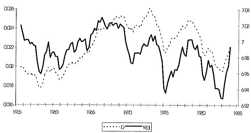
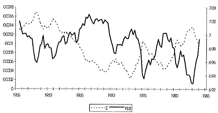
i. Given a vector of parameters and an initial value for we recursively obtain series on , , , and . To do this we make use of a second order approximation to the depreciation function around the steady state and of the competitive equilibrium of the economy. Then, for each period we solve the first-order conditions for maintenance costs (7) and utilization (8) of the planner's problem jointly with the law of motion for the capital stock given series on observed and . We search for an initial value of capital stock such that the average capital-output ratio implied by our resulting capital series is approximately the same that the one obtained from the official capital stock series. Figures 2 and 3 depict observed and model-based time series for and respectively. Figures 5 and 6 show our model-based series for and respectively, and their cyclical behavior with respect to observed and detrended output ( ).
ii. With the observed , and series, and given our measures of and we deduce a time series on effort by solving the optimal condition for effort for each period t
\[\frac {\theta}{(T - \psi - w _ {t} l)} = \frac {\alpha (Y _ {t} + m _ {t} K _ {t})}{C _ {t} w _ {t} h _ {t}}\tag{13}\]
iii. Once unobserved variables as well as those poorly measured variables have been computed, we linearly approximate the technology process for each point in our sample according to
\[\ln (X _ {t}) = [ \ln (Y _ {t} + m _ {t} K _ {t}) - (1 - \alpha) (\ln (K _ {t}) + \ln (u _ {t})) - \alpha (\ln (h _ {t}) + \ln (w _ {t})) ] / \alpha\tag{14}\]
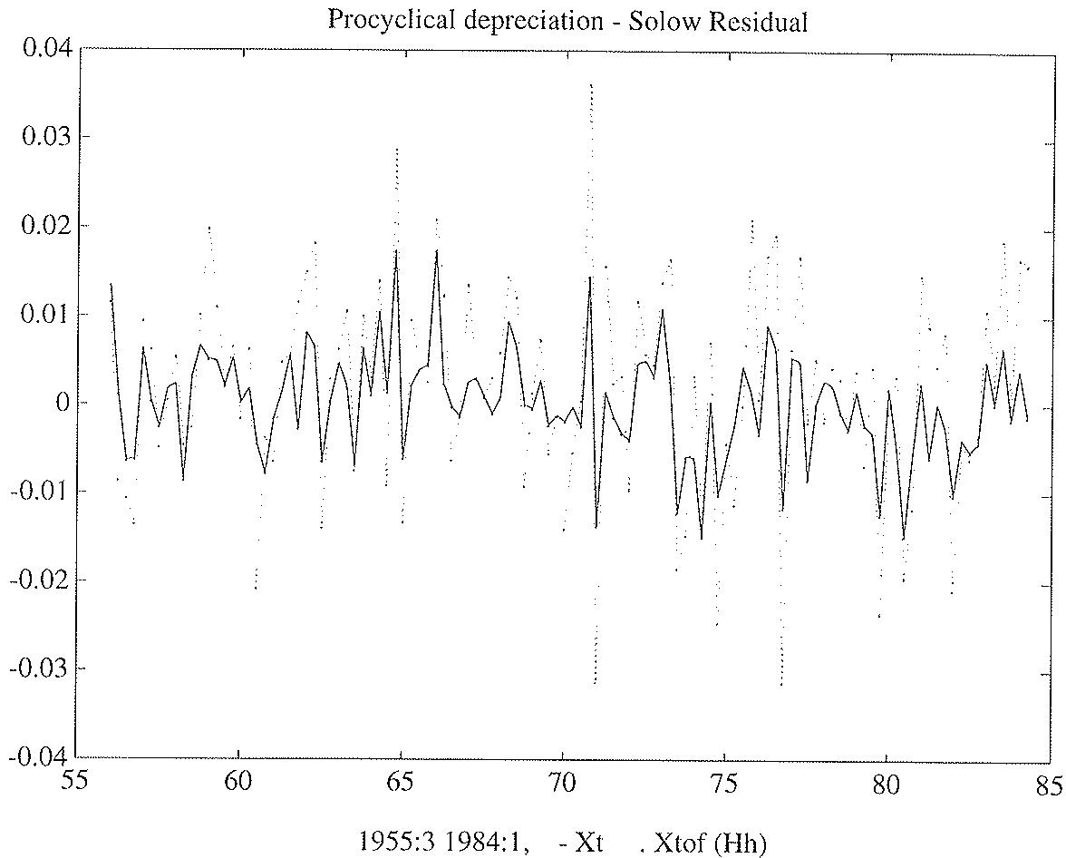
We find that the process is difference stationary and according to equation (3) we interpret the innovation to this process as the true technology shock. Time series for the Solow residual and our measure of technology shocks are depicted in Figure 4. Clearly, our approximate measure of technology shocks is less volatile than the one obtained from the conventional Solow's approach.
5 Findings
Table 2 reports some selected properties of the second moments of Hodrick and Prescott (HP) filtered data for the U.S. economy and for two model economies: column 2 summarizes the results obtained by Burnside and Eichenbaum (1994) under the depreciation in use assumption, and column 3 reports our results. From these results it can be stated that the selected parameters of the depreciation function fits well our targeted second moments properties. The standard deviation of HP filtered output of the model economy approximates the corresponding one generated by U.S data, which stresses on the contribution of productivity shocks to the propagation of aggregate fluctuations.
Table 3 reports our measure of the propagation mechanism for the two models under consideration. As we expected from our results in section 3, with countercyclical maintenance costs we find that the standard deviation of output is more than twice the standard deviation of the technology shock. This statistic is larger than the corresponding one obtained when just the depreciation in use assumption is under consideration. Thus, we conclude that incorporating the existence of countercyclical maintenance costs gives rise to a quantitatively important source of propagation to aggregate technology shocks.
In this case, the standard deviation of the HP filtered level of technology is roughly a 30% less than the one obtained under the depreciation in use assumption. Furthermore, when we compare our results with a standard real business cycle model as the one studied by Christiano and Eichenbaum (1992), in which technology shocks are measured by the Solow residual and it is assumed the same process for technology shocks, we find that the standard deviation of our innovation to technology is nearly a 60% less.
6 Concluding remarks
In this paper we quantify the role played by variable capital utilization rates and maintenance costs in propagating technology shocks over the business cycle. To this purpose we model a depreciation technology depending both on the utilization rate and the maintenance rate. Following part of the literature we assume that using capital increases the rate at which capital depreciates. In addition, we argue that the maintenance activity must be countercyclical, because it is cheaper for the firm to repair and maintain machines when they are stopped than when machines are being employed. We find that small innovations to technology induce large fluctuations in output through the procyclicality of effective capital services and the countercyclicality of the maintenance activity. Specifically, under our model specification the volatility of output is more than two times larger than the volatility of our measure of technology shocks. Furthermore, our estimate for the volatility of output is close to the one implied by U.S. data.
These findings support the traditional argument of the real business cycles literature that fluctuations in technical progress can account for a large fraction of observed fluctuations in aggregate economic time series. Further explorations are necessary to evaluate the behavior of the model in accounting for additional features of observed business cycles and to build evidence either confirming or rejecting our hypothesis. We view the model considered in this paper as a first approximation to richer environments incorporating a completely specified depreciation technology jointly with the role played by utilization rates in determining the effective capital services. We conclude that there is much to be learned from the explicit modeling of the underemployment of production factors.
References
- Bils, M. and Cho, J. (1994), “Cyclical Factor Utilization” Journal of Monetary Economics, Vol. 33, 319-354.
References
- Bresnahan, T. F. and Ramey, V. A. (1993), “Segment Shifts and Capacity Utilization in the U.S. Automobile Industry,” American Economic Review, 83, 213-218.
References
- Burnside, C., Eichenbaum, M. and Rebelo, S. (1993), “Labor Hoarding and the Business Cycle,” Journal of Political Economy, Vol. 101, 245-273.
References
- Burnside, C. and Eichenbaum, M. (1994), “Factor Hoarding and the Propagation of Business Cycle Shocks,” NBER Working Paper # 4675.
References
- Castañeda, A., Díaz-Giménez, J. and Rios-Rull, V. (1995), “Unemployment Spells and Income Distribution Dynamics,” Working Paper 95-10, Universidad Carlos III de Madrid.
References
- Christiano, L. J. (1987), Technical appendix to “Why Does Inventory Investment Fluctuates So Much?,” Working Paper 380, Federal Reserve Bank of Minneapolis.
References
- Christiano, L. J. (1988), “Why Does Inventory Investment Fluctuates So Much?,” Journal of Monetary Economics, 21, 247-280.
References
- Christiano, L. and Eichenbaum, M. (1992), “Current Real Business Cycle Theories and Aggregate Labor Market Fluctuations,” American Economic Review, 82, 430-450.
References
- Cochrane, J. (1994), “Shocks,” NBER Macroeconomics Annual, 141-219.
References
- Cooley, T. F., Hansen, G. D. and Prescott, E. C. (1994) “Equilibrium Business Cycles with Idle Resources and Variable Capital Utilization,” Research Department, Federal Reserve Bank of Minneapolis. Working Paper 535.
References
- Cooley, T. F. and Prescott, E. C. (1995), “Economic Growth and Business Cycles”. Chapter 1 of Frontiers of Business Cycle Research, ed. T. Cooley. Princeton University Press.
References
- Fagnart, J-F, Licandro, O. and Sneessens, H.R. (1995), “Capacity Utilization Dynamics and Market Power,” Universidad Carlos III de Madrid. Working Paper 95-15.
References
- Greenwood, J., Hercowitz, Z., and Huffman, W. (1988), “Investment, Capacity utilization and the Real Business Cycle,” American Economic Review, 78, 402-417.
References
- Greenwood, J., Hercowitz, Z., and Krusell, P. (1992), “Macroeconomic Implications of Investment-Specific Technological Change,” Institute for International Economic Studies, Seminar Paper No. 527.
References
- Hansen, G. (1985) “Indivisible Labor and the Business Cycle” Journal of Monetary Economics, Vol. 16, 309-328.
References
- Hansen, G. (1989) “Technical Progress and Aggregate Fluctuations”, UCLA, mimeo.
References
- King, R., Plosser, C. and Rebelo, S. (1988), “Production, Growth and Business Cycles,” Journal of Monetary Economics, Vol. 21, 195-232, 309-341.
References
- Kydland, F. and Prescott, E. C. (1982), “Time to Build and Aggregate Fluctuations,” Econometrica 50, 1345 - 1370.
References
- Kydland, F. and Prescott, E. C. (1991), “Hours and Employment Variation in Business Cycle Theory,” Economic Theory 1, 63-81.
References
- Rogerson, R. (1988), “Indivisible labor, lotteries and equilibrium,” Journal of Monetary Economics 21, 3-16.
References
- Shapiro, M. D. (1989) “Assessing the Federal Reserve’s Measures of Capacity and Utilization,” Brookings Papers on Economic Activity, 1, 181-241.
Table 1: Calibrated economy's parameters.
| Preferences | ||
| Individual's time endowment | $T$ | 1369 hours per quarter |
| Annual real interest rate | $r$ | 3%; $\beta = 1.03^{-1/4}$ |
| Fixed cost to go to work | $\psi$ | 60 hours |
| Preference for leisure | $\theta$ | 3.5403 |
| Steady state effort | $\bar{w}$ | 1 |
| Shift length | $l$ | 324.7775 hours |
| Steady state employment | $\bar{n}$ | 0.9863 |
| Technology | ||
| Average labor share | $\alpha$ | 0.6210 |
| Average depreciation rate | $\delta$ | 0.0209 |
| Average rate of growth | $\gamma$ | 0.0040 |
| Average utilization rate | $u$ | 0.82 |
| Capital-output ratio | $k/y$ | 10.566 |
| Steady state maintenance | $\bar{m}$ | 0.0021 |
| Shares of output | ||
| Consumption share | $c/y$ | 0.5512 |
| Investment share | $i/y$ | 0.2710 |
| Government share | $g/y$ | 0.1778 |
| Depreciation function | ||
| First derivatives: | $\delta_u$ | 0.042 |
| $\delta_m$ | -1 | |
| Second derivatives: | $\delta_{mu}$ | 3.1 |
| $\Omega$ | 0.21 | |
| $\phi$ | 0.545 | |
Table 2: Second moments properties for HP detrended data. Statistics for the models are averages of 1000 simulations, each of 115 observations length.
| Moment | U.S. data | Depreciation in use model | Maintenance costs model |
| $\sigma_c/\sigma_y$ | 0.427 | 0.453 | 0.422 |
| $\sigma_i/\sigma_y$ | 2.193 | 2.224 | 2.154 |
| $\sigma_h/\sigma_y$ | 0.841 | 0.757 | 0.526 |
| $\sigma_h/\sigma_{y/n}$ | 1.218 | 1.171 | 0.995 |
| $\sigma_y$ | 0.0192 | 0.0167 | 0.0178 |
Table 3: Propagation mechanism for HP detrended data.
| Moment | Depreciation in use model | Maintenance costs model |
| $\sigma_z$ | 0.0114 | 0.0076 |
| $\sigma_y/\sigma_z$ | 1.4670 | 2.3330 |
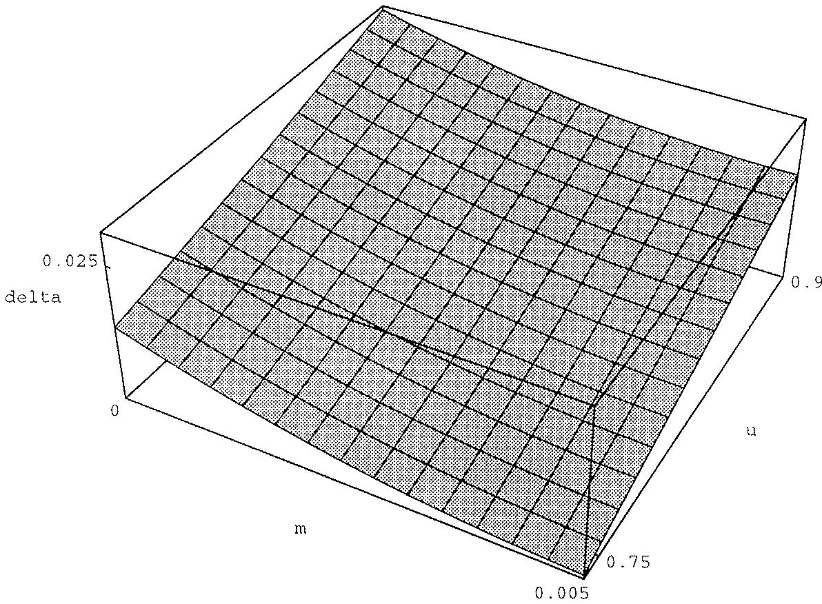
Figure 2: Measures of capital. Official and Model-Based (solid line) series.
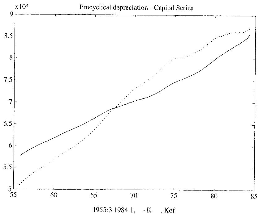
Figure 3: Measures of utilization. Official and Model-Based (solid line) series.
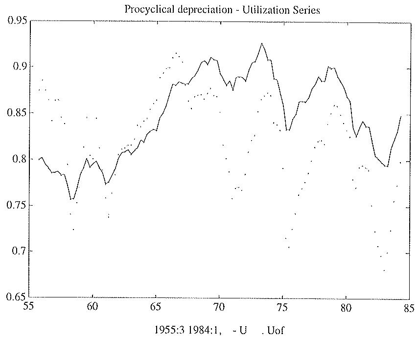
Figure 4: Measures of technology shocks. Solow residual and Model-Based (solid line) series.
Procyclical Depreciation - Depreciation and Output series Figure 5: Cyclical behavior of depreciation. Model-Based depreciation and observed output series.
Procydical Depreciation - Maintenance and Output series Figure 6: Cyclical behavior of maintenance costs. Model-Based maintenance costs and observed output series.
Departamento:
Persona de contacto:
Código Postal: Población: Capital:
Teléfono: Fax:
Deseo recibir regularmente:
[ ] Documentos de trabajo
[ ] Boletín
Deseo recibir el Documento de Trabajo N°.....
Deseo recibir en diskette el D.T. N ....
Remitir esta solitud a:
FEDEA - Documentación
Jorge Juan, 46
28001 MADRID
Fax: (91) 577 95 75
Telf.: (91) 435 90 20
* Indicar el documento de trabajo deseado (a partir del n° 94-05). Se enviará un diskette que contenga el texto de dicho documento en formato WPD (Word Perfect versión 6.0), para su reproducción en tamaño DIN A4.
DOCUMENTOS DE TRABAJO
References
- 94-15: "Profitability of the different services of RENFE", John Dodgson y Pablo Rodríguez.
References
- 94-16: "Exchange rate volatility in the EMS before and after the fall", Simón Sosvilla-Rivero, Fernando Fernández-Rodríguez, Oscar Bajo-Rubio y Juan Martín-González.
References
- 94-17: "Consecuencias socio-económicas de las tendencias demográficas españolas", José A. Herce.
References
- 94-18: "Efectos de la desregulación del transporte aérero en España", Ofelia Betancor y J. D. Jorge Calderón.
References
- 94-19: "Regulación de las oficinas de Farmacia: Precios y libertad de entrada", Walter García-Fontes y Massimo Motta.
References
- 94-20: "Irreversibility, uncertainty and underemployment equilibria", David de la Croix y Omar Licandro.
References
- 95-01: "Workforce adjustment in Spain: Are working hours a choice variable?*, Carlos García-Serrano, Juan F. Jimeno and Luis Toharia.
References
- 95-02: "The organization of bargaining in Spanish firms", Diego R. Palenzuela y Juan F. Jimeno.
References
- 95-03: "Las pensiones públicas en España: Perspectivas y posibilidades de reforma", José A. Herce.
References
- 95-04: "Structural unemployment. Spain versus Portugal", Olivier Blanchard y Juan F. Jimeno.
References
- 95-05: ""Review of the regulation of road freight in the UK", G. Tweddle y P. J. Mackie.
References
- 95-06: "Efectos de la desregulación del transporte de mercancía por carretera", Anna Matas, (Ayudantes de Investigación: Bienvenido Ortega y Jesús Prado).
References
- 95-07: "Capacity utilization dynamics and market power", J-F. Fagnart, O. Licandro y H.R. Sneessens.
References
- 95-08: "Creative destruction and business cycles", Raouf Boucekkine, Marc Germain, Omar Licandro.
References
- 95-09: "Regional Unemployment Persistence (Spain, 1976-1994)", Juan F. Jimeno y Samuel Bentolila.
References
- 95-10: " A quantitative analysis of the effects of capital control: Spain 1986-1990", Oscar Bajo-Rubio and Simón Sosvilla Rivero.
References
- 95-11: "La Asignación del espacio en los aeropuertos", Juan Pablo Nicolini y Ricard Torres.
References
- 95-12: "Regulación de la innovación tecnológica en el mercado sanitario: Una valoración de la efectividad de los instrumentos", Jaume Puig i Junoy y Eulàlia Dalmau i Matarradona.
References
- 95-13: "La financiación pública de los servicios sanitarios en España", Beatriz González López-Valcárcel, Laura Pellisé Urquiza y Patricia Barber Pérez.
References
- 95-14: "Patrones territoriales de crecimiento industrial en España", Ana Goicolea, José A. Herce y Juan J. de Lucio.
References
- 94-15: "Análisis de la rentabilidad social de proyectos de inversión en infraestructuras de transporte del Marco de Apoyo Comunitario 1989-93", Ginés de Rus Mendoza y Manuel Romero Hernández.
References
- 95-16: Capital utilization, maintenance costs and the business cycle", Omar Licandro y Luis A. Puch.
Este texto se ha extraído automáticamente del documento original. Para citarlo o leerlo con su maquetación, descargue el PDF.
Descargar en PDF