Idiosyncratic uncertainty, capacity utilization and the business cycle por J-Fr. Fagnart*, O. Licandro** and Franck Portier***
DOCUMENTO DE TRABAJO 96-11
Abril, 1996
* University of Copenhagen and Université Catholique de Louvain
** FEDEA and Universidad Carlos III de Madrid
*** CEPREMAP, MAD and Université de Rouen
Jean-François Fagnart, Omar Licandro and Franck Portier *
First version: April 1995 This version: February 1996
Abstract
In a stochastic dynamic general equilibrium framework, we introduce the concept of variable capacity utilization (as opposed to the concept of capital utilization). We consider an economy where imperfectly competitive firms use a putty-clay technology and decide on their productive capacity level under uncertainty. An idiosyncratic uncertainty about the exact position of the demand curve faced by each firm explains why some productive capacities may remain idle in the sequel and why individual capacity utilization rates differ across firms. The capacity underutilization at the aggregate level thus hides a diversity of microeconomic situations. The variability of the capacity utilization allows for a good description of some of the main stylized facts of the business cycle, propagates and magnifies aggregate technological shocks and generates endogenous persistence (i.e., the output growth rate displays positive serial correlation).
1 Introduction
The fact that the entire stock of capital is never fully used for production is now recognized as an important element in the understanding of the business cycle fluctuations. There is however no consensus in the literature on the way of modeling this underutilization phenomenon.
A first strand of the literature (Greenwood, Hercowitz and Huffman [1988], Burnside and Eichenbaum [1994], Licandro and Puch [1995]) introduces a capital utilization variable by assuming that the capital depreciation rate is a function of the capital utilization rate. In such “depreciation in use” models, the concept of production capacity is not relevant as such: it is the intensity of the period of time with which a unit of capital is utilized that varies (the intensive margin). Strictly speaking -and contrary to what is often done in that literature, such a capital utilization concept cannot be compared to the Federal Reserve’s measure of capacity utilization. As Burnside and Eichenbaum [1994] recognize, the “depreciation in use” assumption should be viewed as a very crude approximation of the multiple means that firms use to regulate their production. In particular, this assumption is not directly compatible with the microeconomic evidence on the underutilization phenomenon reported by Bresnahan and Ramey [1993]. On the basis of data from the automobile industry, the latter authors show that the most usual way of adjusting production is to vary regular hours by shutting the plant down for a week. This phenomenon of capacity idleness is not taken into account per se by the “depreciation in use” models.
*J-F. Fagnart, University of Copenhagen and Université Catholique de Louvain. O. Licandro, FEDEA and Universidad Carlos III de Madrid. F. Portier, CEPREMAP, MAD and Université de Rouen. We thank Pierre Malgrange for his very detailed comments on an earlier draft and the participants at the MAD-University of Paris I, Maastricht-HCM and Copenhagen workshops. We gratefully acknowledge the financial support of the Commission of the European Union (contract ERBCHRXCT940658) and the Ministry of Scientific Research of the Belgian French Speaking Community (PAC 62-93/98)
A second strand of the literature (Kydland and Prescott [1988], Bils and Cho [1994]) assumes that the utilization rate of capital increases when employees work at a higher level of effort. Again, these models cannot account for idle units of capital: it is only the intensity of the period of time with which a unit of capital is utilized that varies.
The third strand of the literature introduces explicitly a variable capacity utilization within a real business cycle model. As far as we know, this strand is only represented by Cooley, Hansen and Prescott [1995]. In their model, production takes place at the level of individual plants, which face idiosyncratic technological shocks. Operating a plant implies a fixed cost. Depending on the idiosyncratic shock (s)he observes, the plant manager must thus decide whether to operate the plant (and to bear the fixed cost) or to leave the plant idle. The macroeconomic equilibrium is characterized by a variable proportion of operating plants. The paper concludes that, except for variations in factors share in value added, the cyclical properties of the model are close to the ones of a standard real business cycles economy. Moreover, the introduction of a variable capacity utilization does not increase the internal propagation mechanisms of the model: a more variable aggregate technological shock is even required to reproduce the output variability.
A priori, the conclusion of Cooley, Hansen and Prescott [1995] thus casts some doubt on the conjecture of Burnside and Eichenbaum [1994] who suggest that a model with explicit capacity underutilization should produce the same type of results as theirs (i.e., variable capital utilization rate substantially magnifies and propagates the impact of shocks to agents' environments). In a stochastic general equilibrium model that extends a model developed by Sneessens [1987], Licandro [1995] and Fagnart, Licandro and Sneessens [1995], we show that variable capacity utilization can play an important role in magnifying and propagating aggregate (technological) shocks, contrary to the conclusion of Cooley, Hansen and Prescott [1995]. This suggests that the results of Burnside and Eichenbaum [1994] can remain true in a model that allows explicitly for idle capacities.
The model we propose relies on three basic intuitions: (i) the very concept of productive capacities suggests that in the short run, the possibilities of substitution between production factors are very limited; (ii) given this technological rigidity, the presence of uncertainty at the time of installing productive equipment may explain why production capacities are usually underutilized at the aggregate level; (iii) idiosyncratic uncertainty and imperfect competition in the goods market can explain why, as reported in business surveys, some firms produce at full capacity while others face demand shortages and underuse capital.
The model consists of a competitive sector producing a final good and a monopolistic sector producing intermediate goods. In the intermediary sector, we introduce a technological rigidity by assuming a putty-clay technology: capital and labor are substitute ex ante (i.e., before investing) but complement ex post (i.e., once equipment are installed) . Moreover, each intermediate firm sets its price under (idiosyncratic) uncertainty about the exact position of its demand curve. Since the stock of capital and the capital-labor ratio are given at period t, the production of the monopolistic firm can be constrained by either its installed productive capacity or sales shortages. The general equilibrium is therefore non-symmetric in quantities: some firms face demand shortages and have excess capacities while the others are at full capacity and cannot satisfy any extra demand. The model is closed by introducing an infinitely living consumer-worker.
Our model with variable capacity utilization propagates and magnifies aggregate technological shocks. It describes in a satisfactory way some of the main stylized facts of the business cycle. Moreover the artificial business cycle displays a positive serial correlation of output growth rate.
The paper is organized as follows: section 2 describes the model, section 3 discusses the calibration, section 4 presents the results and section 5 concludes.
2 The Model
2.1 Consumers
We suppose identical and infinitely living consumers whose preferences at date t ( ) are represented by a time separable utility function defined over consumption and labor:
\[U _ {t} = \operatorname{E} _ {t} \left[ \sum_ {s = 0} ^ {\infty} \beta^ {s} \left(\log (C _ {t + s}) + v (1 - L _ {t + s})\right) \right]\]
with , . In the sequel, represents the elasticity of . represents the expectation operator given the information available at date t. and are the consumption and labor supply at that date. is a constant subjective discount rate.
The representative household enters into period t with a predetermined level of nominal financial assets ( is given). During the period, she receives a wage income, firms' profits and the remuneration of her financial assets. Let , and
E.g.
E.g. this may be the case simply because implementing these substitutions requires time.
Our putty-clay assumption is thus roughly modeled. We only assume that capital stock and capital labor ratio are predetermined variables. There is no vintage of capital in the model.
represent the nominal price of consumption, the nominal wage rate and the nominal interest rate. At date , the budget constraint of the household is given by:
\[A _ {t + 1} \leq (1 + R _ {t}) A _ {t} + W _ {t} L _ {t} + \Pi_ {t} - \mathcal {P} _ {t} C _ {t}.\tag{1}\]
where is predetermined and and are taken as given.
At each date t, the representative household chooses and in order to maximize subject to (1). The first order conditions for and are given by
\[w _ {t} = v ^ {\prime} (1 - L _ {t}) C _ {t}\tag{2}\]
\[{\frac {1}{C _ {t}}} = {\beta \operatorname{E} _ {t} \left[ \frac {\rho_ {t + 1}}{C _ {t + 1}} \right]}\tag{3}\]
where is the real wage rate (i.e., ) and is 1 plus the real interest rate (i.e., ).
2.2 Final Good Sector
This section follows Fagnart, Licandro and Sneessens [1995]. There is a single final good produced by a representative firm. This final good is sold on a competitive market and can be used for consumption or investment.
The production technology is represented by a constant returns-to-scale CES function defined over a continuum of variable inputs in the interval . The quantity of each input is represented by y and indexed by j. More formally, the representative firm's output (denoted Y) is obtained from the following production function:
\[Y _ {t} = \left[ \int_ {0} ^ {1} v _ {t} ^ {j \frac {1}{\theta}} y _ {t} ^ {j \frac {\theta - 1}{\theta}} \mathrm{d} j \right] ^ {\frac {\theta}{\theta - 1}}.\tag{4}\]
Each productivity parameter is drawn from an i.i.d. distribution function with unit mean. In the sequel, we will assume a lognormal distribution function. The parameter will represent the standard deviation of the logarithm of .
The firm purchases inputs in the intermediate goods sector. The total supply of input j is limited to an amount (see below), equal to the productive capacity of the corresponding input supplying firm. When maximizing its profit function, the final firm faces no uncertainty: it knows the inputs prices , the supply constraints and the productivity parameters . Moreover, it takes the final output price as given. The optimization program of the firm is then:
\[\max _ {\{y _ {t} ^ {j} \} _ {j}} \mathcal {P} _ {t} Y _ {t} - \int_ {0} ^ {1} P _ {t} ^ {j} y _ {t} ^ {j} \mathrm{d} j\]
\[\text { subject to the supply constraints } \quad y _ {t} ^ {j} \leq q _ {t} ^ {j} \quad \forall j \in [ 0, 1 ]\]
where is defined by (4). Notice the presence of the input supply constraints in the optimization program of the final firm. Since the input prices are set in advance, the final firm has indeed to take into account that some inputs may be in short supply. If this is the case, it is profitable for the final firm to make appropriate inputs substitutions, i.e., to modify its demands for the unconstrained inputs.
Let be the relative price of input with respect to the final good price:
\[p _ {t} ^ {j} = \frac {P _ {t} ^ {j}}{\mathcal {P} _ {t}} \quad \forall j \in [ 0, 1 ].\]
The solution to the above maximization problem can be described by the following system of equations
\[y _ {t} ^ {j} = \left\{ \begin{array}{l l} {\left(p _ {t} ^ {j}\right) ^ {- \theta} Y _ {t} v _ {t} ^ {j}} & \mathrm{if} v _ {t} ^ {j} \leq \widetilde {v} _ {t} ^ {j} \\ q _ {t} ^ {j} & \mathrm{if} v _ {t} ^ {j} \geq \widetilde {v} _ {t} ^ {j} \end{array} \right. \quad \forall j \in [ 0, 1 ]\tag{5}\]
where the critical value of the productivity parameter, , is such the demand for j at relative price is equal to the production capacity of supplier j, i.e.,
\[\widetilde {v} _ {t} ^ {j} = \frac {q _ {t} ^ {j}}{\left(p _ {t} ^ {j}\right) ^ {- \theta} Y _ {t}}.\tag{6}\]
A Clower constraint on final good transactions, as in King [1990] or Magill and Quinzii [1992], is assumed in each period:
\[\mathcal {P} _ {t} Y _ {t} = \overline {{M}}\tag{7}\]
where is a fixed quantity of money. This equation determines the nominal price level .
2.3 Intermediate Inputs Sector
Each input j is produced by a single firm in a monopolistically competitive market.
j
It is worth outlining how the binding supply constraints affect the demands for the unconstrained inputs. When no constraint is binding, the input demand functions are all linear in the final output level (see (5) where ). So is the cost function of . The marginal cost of is thus a function (or an index) of the input prices only. At given final output level, the demand for input j thus depends on the ratio of the price of j and the above mentioned price index (also equal to the final price given the competitive behavior of the final firm). Things becomes more complicated when some inputs are in short supply. The induced substitutions between inputs imply indeed an increase in the marginal cost of a given output level. Consequently, the marginal cost of the final output depends not only on the input prices but also on the importance of the supply constraints (and so on the final output level itself). In other words, binding input constraints makes returns-to-scale decreasing. At the output level which satisfies the equality between marginal cost and the final good price , the demands for the unconstrained inputs are thus affected in two ways. On the one hand, binding supply constraints induce substitutions Favorable to the unconstrained inputs. On the other hand, binding supply constraints also reduce the optimal output level and so the demand for the unconstrained inputs.
2.3.1 Individual Firm's Problem
Putty-Clay Technology: We assume that each input firm uses a “putty-clay” technology but we want to model this idea in the simplest way.
Investments achieved during period t - 1 become productive at date t. When investing in t - 1, a firm chooses simultaneously the future capital stock and the capital-labor ratio embodied in the productive equipment used during period t ( and are given). When investing, the firm can thus substitute capital for labor by choosing the optimal ratio between the two factors in the production process. Once the equipment are installed, modifying x requires new investments and (one period of) time.
Assuming a Cobb-Douglas technology, the average productivities of labor and capital are respectively and , with . At each date t, the aggregate productivity parameter, , obeys the following stochastic process:
\[\log \alpha_ {t} = \phi \log \alpha_ {t - 1} + \epsilon_ {t}\tag{8}\]
where and are i.i.d. innovations with standard deviation .
Once the capital is installed, the productive capacity of firm j is given by
\[q _ {t} ^ {j} = \alpha_ {t} (x _ {t} ^ {j}) ^ {\eta - 1} k _ {t} ^ {j}.\tag{9}\]
As stated before, modifying the capital-labor ratio takes one period and requires an amount of technical investment given by where and . Finally, we assume that each firm has to bear a fixed cost of production .
Decision Sequence: From each input firm's point of view, two exogenous variables exhibit a random behavior: the aggregate productivity parameter and the idiosyncratic productivity shock , which is perceived as a demand shock by the input firm. During time period , firm takes three types of decisions.
After having observed , but under demand uncertainty, it sets its nominal price . Note that the knowledge of allows the firm to compute the equilibrium values of all the aggregate variables at date t since the uncertainty at this stage is purely idiosyncratic.
Once all the uncertainty is resolved, firm j observes its demand and produce a quantity given by (5). Labor is supposed to be a purely variable input. It is bought on a competitive market and labor demand can be adjusted instantaneously to the production plan :
\[\ell_ {t} ^ {j} = \frac {y _ {t} ^ {j}}{\alpha_ {t} ^ {j} (x _ {t} ^ {j}) ^ {\eta}}.\tag{10}\]
Eventually, the input firm decides on the productive capital stock and the technology .
This assumption will allow us to reduce the value of pure profits in the calibration of the model.
Optimization Program : At date t, the maximization problem that summarizes the above decision sequence may be written as follows
\[\max \left. \right. \mathrm{E} _ {t} \left[ \sum_ {s = 0} ^ {\infty} \left(P _ {t + s} ^ {j} y _ {t + s} ^ {j} - W _ {t + s} \ell_ {t + s} ^ {j} - \mathcal {P} _ {t + s} \left(k _ {t + s + 1} ^ {j} - (1 - \delta) k _ {t + s} ^ {j} + \Psi (\Delta x _ {t + s + 1} ^ {j}) + \Phi\right)\right) \Lambda_ {s} \right]\]
where and are predetermined, and are given by (5) and (10), is the depreciation rate of capital. represents the discount factor, i.e., and
\[\Lambda_ {s} = \prod_ {i = 1} ^ {s} (1 + R _ {i}) ^ {- 1}.\]
For the derivation of the optimality conditions, it is useful to note that expected output, conditional on aggregate information, can be expressed as
\[\mathrm{E} _ {t} (y _ {t} ^ {j}) = (p _ {t} ^ {j}) ^ {- \theta} Y _ {t} \int_ {0} ^ {\widetilde {v} _ {t} ^ {j}} v \mathrm{dF} (v) + q _ {t} ^ {j} \int_ {\widetilde {v} _ {t} ^ {j}} ^ {\infty} \mathrm{dF} (v)\tag{11}\]
where is given by (6) and denotes the lognormal cumulative distribution function.
In order to simplify some expressions, let denote the ratio
\[\pi_ {t} ^ {j} = \frac {(p _ {t} ^ {j}) ^ {- 0} Y _ {t} \int_ {0} ^ {\widetilde {v} _ {t} ^ {j}} v \mathrm{dF} (v)}{\mathrm{E} _ {t} (y _ {t} ^ {j})}.\tag{12}\]
represents the elasticity of expected output with respect to (i.e., the demand firm j can expect in case of idle capacities). Alternatively, this elasticity can be interpreted as the (weighted) probability of capacity underutilization. It is necessarily smaller than 1.
Taking into account that aggregates are perfectly foreseen when firm j sets its price, the first order condition with respect to may be written as
\[P _ {t} ^ {j} = \mu_ {t} ^ {j} \frac {W _ {t}}{\alpha_ {t} (x _ {t} ^ {j}) ^ {\eta}} \quad \mathrm{where} \quad \mu_ {t} ^ {j} = \frac {\theta \pi_ {t} ^ {j}}{\theta \pi_ {t} ^ {j} - 1}.\tag{13}\]
The optimality condition on implies a margin over the marginal cost of production. This margin depends negatively on the weighted probability of capacity underutilization .
The optimality condition for the capital stock is
\[\mathrm{1-} \mathrm{E} _ {t} \left[ \frac {1 - \delta}{\rho_ {t + 1}} \right] = \mathrm{E} _ {t} \left[ \frac {1}{\rho_ {t + 1}} \underbrace {\left(\frac {p _ {t + 1} ^ {j}}{\theta \pi_ {t + 1} ^ {j}}\right)} _ {(A)} \alpha_ {t + 1} (x _ {t + 1} ^ {j}) ^ {\eta - 1} (1 - \mathrm{F} (\widetilde {v} _ {t + 1} ^ {j})) \right]\tag{14}\]
The optimal capital stock is given by the equality between the net cost of installing 1 unit of capital at date t (given its depreciation rate per time period) and the expected marginal revenue of this unit at date . The expected marginal revenue is equal to the profit margin per unit of output (A), times the physical productivity of capital , times the probability of using the marginal unit of capital . Finally, the marginal condition for is
\[\begin{array}{r c l} \Psi \Delta x _ {t + 1} ^ {j} & = & \mathrm{E} _ {t} \left[ \frac {\Psi \Delta x _ {t + 2} ^ {j}}{\rho_ {t + 1}} \right] - \mathrm{E} _ {t} \left[ \frac {1}{\rho_ {t + 1}} \underbrace {(1 - \eta) p _ {t + 1} ^ {j} \frac {q _ {t + 1} ^ {j}}{x _ {t + 1} ^ {j}}} _ {(A ^ {\prime})} (1 - \mathrm{F} (\widetilde {v} _ {t + 1} ^ {j})) \right] \\ & + & \mathrm{E} _ {t} \left[ \frac {1}{\rho_ {t + 1}} \underbrace {w _ {t + 1} \left(\frac {\eta}{\widetilde {v} _ {t + 1} ^ {j}} \int_ {0} ^ {\widetilde {v} _ {t + 1} ^ {j}} v \mathrm{dF} (v) + 1 - \mathrm{F} (\widetilde {v} _ {t + 1} ^ {j})\right) \frac {k _ {t + 1} ^ {j}}{(x _ {t + 1} ^ {j}) ^ {2}}} _ {(B ^ {\prime})} \right]. \end{array}\tag{15}\]
Given the investment cost in technical change, the optimal capital-labor ratio is raised up to value at which the expected decrease in sales due to the lower productivity of capital (A') when the capacity constraint is binding (what occurs with a probability ) is equal to the reduction in labor costs resulting from the higher productivity of labor at any production level (B').
2.3.2 Equilibrium in the Inputs Sector and Aggregation
When investing in t-1, all firms have the same information regarding the future. They thus choose the same capital stock and capital-labor ratio:
\[k _ {t} ^ {j} = k _ {t} \quad \mathrm{and} \quad x _ {t} ^ {j} = x _ {t}, \quad \forall t \geq 0, \forall j \in [ 0, 1 ]\]
Consequently, , for all .
At the time of setting prices, they have the same information regarding the aggregate and individual demands. They thus announce the same price since they have the same productive capacity: . The relative price between any input and the final good is then
\[p _ {t} = \frac {P _ {t}}{\mathcal {P} _ {t}} < 1.\]
As we have explained in footnote 3, the inequality between and follows from the presence of binding capacity constraints, which raise the marginal cost and the price of the final output at given input prices.
In the symmetric equilibrium described above, the critical value is thus the same for all firms and is denoted . Ex post (i.e., once all the uncertainty is resolved), input firms experience different idiosyncratic shocks and are in heterogeneous situations. The actual output level in firm j is then:
\[y _ {t} ^ {j} = \left\{ \begin{array}{l l} (p _ {t}) ^ {- \theta} Y _ {t} v _ {t} ^ {j} & \text {if} v _ {t} ^ {j} \leq \widetilde {v} _ {t} \\ q _ {t} & \text {if} v _ {t} ^ {j} \geq \widetilde {v} _ {t} \end{array} \right. \quad \forall j \in [ 0, 1 ]\tag{16}\]
We extend the symmetry assumption to initial conditions.
Note that the demand served by a firm underusing its productive capacity (i.e., any firm j for which ) is : it is only in absence of binding supply constraints that would represent the demand for j at a symmetric equilibrium in input prices. The term measures the spillover effect coming from the binding supply constraints.
Aggregate employment, denoted , is equal to the sum of the individual employment levels, i.e.,
\[L _ {t} = \frac {p _ {t} ^ {- \theta} Y _ {t}}{\alpha_ {t} x _ {t} ^ {\eta}} \int_ {0} ^ {\widetilde {v} _ {t}} v \mathrm{dF} (v) + \frac {k _ {t}}{x _ {t}} \int_ {\widetilde {v} _ {t}} ^ {\infty} \mathrm{dF} (v)\tag{17}\]
From (4) and (5), the final output supply is given by:
\[Y _ {t} = \left\{\left[ p _ {t} ^ {- \theta} Y _ {t} \right] ^ {\frac {\theta - 1}{\theta}} \left[ \int_ {0} ^ {\widetilde {v} _ {t}} v \mathrm{dF} (v) \right] + \left(q _ {t}\right) ^ {\frac {\theta - 1}{\theta}} \left[ \int_ {\widetilde {v} _ {t}} ^ {\infty} v ^ {\frac {1}{\theta}} \mathrm{dF} (v) \right] \right\} ^ {\frac {\theta}{\theta - 1}}\tag{18}\]
where is defined by (6).
At each date, the aggregate productive capacity is underutilized. The underutilization rate is given by
\[D _ {t} = \frac {Y _ {t}}{\bar {s} \alpha_ {t} x _ {t} ^ {\eta - 1} k _ {t}} \leq 1\tag{19}\]
where represents an aggregation constant and can be obtained from . The proportion of firms that underutilize their production capacity is given by . The relative weight of the production of those firms in total production is measured by .
2.4 General Equilibrium and Stationary State Analysis
Given the predetermined variables and , a general equilibrium of the economy at date is characterized by: 1) a symmetric equilibrium in prices, capital stock and technological choices in the intermediate goods sector ( , and , ) where , and are given by (13), (14) and (15); 2) transactions in each input market described by (16); 3) a vector of prices ( ) such that the final good, money and labor markets clear.
We consider now the non-stochastic steady state equilibrium of the above economy, i.e., the economy without aggregate uncertainty but with microeconomic uncertainty. The stationary interest rate is given by the optimal consumption rule, i.e., . At the stationary state, the optimality conditions (13) and (15) on x and p allow us to compute the expression of the weighted proportion of firms that underuse their capacity at the stationary equilibrium:
\[\pi = \frac {1}{1 + (\theta - 1) \eta} < 1.\tag{20}\]
Idiosyncratic uncertainty thus induces necessarily capacity underutilization at the stationary equilibrium . The stationary value of the proportion is decreasing in the degree of substitutability between goods and the elasticity . Larger possibilities of substitution between intermediate goods reduce the effects of the mismatch between inputs demands and supplies, and thus lower the proportion of firms underusing their productive capacity at the equilibrium. Even though the distribution function does not influence the relative weight of the production of firms with excess capacities in total output (see 20), it does affect the equilibrium capacity utilization rate: an increase in the variance of the distribution implies a lower capacity utilization rate at any capacity level.
Under the assumption of lognormality of the idiosyncratic shocks, .
Substituting (see (20)) in conditions (12) and (15) gives an equation for (after some algebraic manipulations):
\[(\theta - 1) \eta \int_ {0} ^ {\widetilde {v}} v \mathrm{d} F (v) = \widetilde {v} \int_ {\widetilde {v}} ^ {\infty} \mathrm{d} F (v).\tag{21}\]
This equation determines as a function of parameters.
By dividing both sides of equation (18) by , one can express the relative price p as a function of :
\[p = \left\{\left[ \int_ {0} ^ {\widetilde {v}} v \mathrm{dF} (v) \right] + (\widetilde {v}) ^ {\frac {\theta - 1}{\theta}} \left[ \int_ {\widetilde {v}} ^ {\infty} v ^ {\frac {1}{\theta}} \mathrm{dF} (v) \right] \right\} ^ {\frac {1}{\theta - 1}}.\tag{22}\]
The optimality condition on may be written as
\[\rho - 1 + \delta = \frac {p}{\theta \pi} x ^ {\eta - 1} (1 - \mathrm{F} (\widetilde {v})).\tag{23}\]
We can thus determine x as a function of . The stationary level of the capital-labor ratio is such that the user cost of one unit of capital is equal to the expected marginal revenue of capital. This expected marginal revenue is equal to the real profit margin per unit of output times the physical productivity of capital, taking into account that it will only be utilized with a probability .
3 Calibration
The model is solved numerically following King, Plosser and Rebelo [1987]. The calibration relies on Cooley, Hansen and Prescott [1995]. We impose restrictions on our artificial economy in order to insure that its non stochastic stationary state is consistent with a list of standard growth facts. That list includes the facts that in U.S. post Korean war data, the average quarterly capital-output ratio is equal to 13.28, investment as a share of output is .25, the share of total income that is paid to capital is .4, the ratio between the average working time and the total available time is .31. These facts determine the values of , , . The parameters and are next chosen in order to reproduce the average capacity utilization rate measured by the Federal Reserve Board of Governors (.82) and to obtain a markup level consistent with the empirical studies for the US industry (Hall [1988], Hall [1990], Morrison [1990]). The fixed cost implies that aggregate pure profits are null, as documented in Rotemberg and Woodford [1995]. The utility of leisure is assumed to be logarithmic, so that . The last point concerns the calibration of aggregate uncertainty. As in
Cooley, Hansen and Prescott [1995], is set to .95. The variance of the innovations is such that the standard deviation of artificial cyclical output is close to the US postwar one.
Table 1: Calibration
| $\eta$ | $\beta$ | $\delta$ | $\theta$ | $\sigma_v$ | $\Phi$ | $\Psi$ | $v_{LL}$ | $\phi$ | $\sigma_\alpha$ |
| .2947 | .9999 | .0188 | 6.0265 | .5384 | 1 | 0 | -1 | .95 | .9% |
The proportion of demand constrained firms at the stationary state equilibrium is equal to . The capital-labor ratio x is 29.48 and the markup level is 1.7.
4 Results
4.1 Impulse Responses to an Aggregate Technological Shock
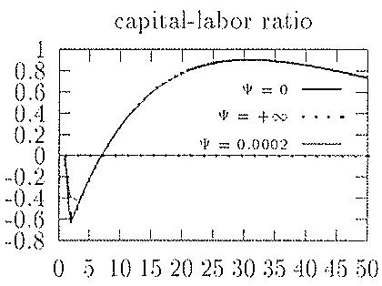
We start this section by analyzing the impulse responses to an aggregate technological shock. . The possibilities of substituting a production factor for the other are likely to play an important role in the response of the model to a technological shock. Consequently, we have wanted to detail the impulse responses of three different versions of the model:
- the Cobb-Douglas case where firms can substitute capital for labor without new technical investments (Case I, ). Firms then use a Cobb Douglas production function with technical coefficients which are fixed during each time period but can be freely modified from one period to the following.
- an intermediary case where firms can substitute capital for labor at the cost of a technical investment. We have chosen a value for that corresponds to the estimation of Bils and Cho [1994] (Case II, ).
- the case where firms cannot substitute capital for labor (Case III, ). Firms then use the same Leontieff technology through time with technical coefficients fixed at their optimal stationary state value.
In the following discussion, we assess whether the presence of idle capacities propagates and magnifies the effects of a technological shock in the economy.
Magnification: Since the technological shock bears on the installed capital stock, it increases ipso facto the productive capacity of firms. Consequently, a rise in capacity utilization will only occur if the output increase is larger than the productivity gain. This effect is observed during the first period in the three artificial economies. Because of consumption smoothing and logarithmic preferences, real wages follow partially the increase in productivity. This reduces the unit labor costs and push real input prices downwards. The resulting increase in demand stimulates output via a more extensive use of productive capacities. It is worth noticing that input prices decrease even though markups increase. In response to a positive technological shock, capacity utilization and markups are procyclical even though real input prices are countercyclical.
These impulse response functions are displayed in appendix.
The instantaneous response of output is different in the three economies. Indeed, the possibility of substituting labor for capital interacts with the labor supply decisions of workers (via their intertemporal arbitrage between leisure to-day and leisure tomorrow). The larger the possibility of substitution between production factors, the more workers are willing to supply labor when its productivity is high in order to work less in the future (when productivity is lower again). This explains the differences in the responses of output, employment, consumption and real wages in the three economies.
Persistence: Since workers increase their labor supply in economies I and II, firms invest initially in a less capital intensive technology (x decreases). During the following period, employment increases accordingly and the one period ahead response of output is greater that the instantaneous one. The resulting hump-shape response of output will account for the positive serial correlation of output growth (see below). This one-period ahead increase is smaller, the larger the adjustment costs on x (Case II). It disappears in the Leontieff economy (Case III).
As far as the responses of the utilization rate, the proportion of firms with idle capacities and the markup rate are concerned, the Cobb Douglas economy (Case I) reacts in a particular way. In absence of any stochastic macroeconomic shock from period 2, each firm is able to modify its capital-labor ratio from one period to the following so as to always maintain the expected capacity utilization rate at its optimal level, given the idiosyncratic demand uncertainty. At the macroeconomic level, this microeconomic behaviors imply that the utilization rate and thus and reach their stationary level from period 2. In the Leontieff economy, adjusting the capital-labor ratio is impossible. Firms thus have to accept a lower expected capacity utilization rate during the adjustment phase.
In summary, the above analysis suggests that the presence of idle capacities magnifies the effects of a global technological shock if the possibilities of technological substitutions between factors are important. This magnification effect is present even though the way we have introduced the aggregate technological shock is not the most favorable to our model: the shock increases the productivity of the installed equipment and allows firms to increase their production without requiring necessarily a more extensive use of existing capacities. A technological shock that would be embodied only in the newly installed equipment, as in Greenwood, Hercowitz and Huffman [1988], would lead to a higher response of the capacity utilization rate. In order to ease the comparison with the literature, we have however assumed a shock on total factor productivity according to the standards of the RBC tradition.
4.2 Simulation Results
All the simulated series have been detrended by using the Hodrick-Prescott filter. The results are obtained from 100 simulations of 150 points each.
Table 2: Cyclical Properties of Actual and Artificial Economies
| Series | S.D. | Cor. with Output | ||||||
| Data | Case I | Case II | Case III | Data | Case I | Case II | Case III | |
| Y | 1.73 | 1.69 | 1.63 | 1.25 | 1 | 1 | 1 | 1 |
| C | .86 | .52 | .51 | .97 | .77 | .95 | .95 | .98 |
| I | 5.34 | 5.57 | 5.37 | 2.74 | .90 | .99 | .99 | .99 |
| L | 1.5 | .80 | .72 | .11 | .86 | .93 | .93 | .84 |
| Y/L | .88 | .99 | 1.01 | 1.16 | .50 | .95 | .96 | .99 |
| wH/Y | .54 | .40 | .42 | .32 | -.32 | -.27 | -.43 | -.53 |
| D | .15 | .15 | .12 | .27 | .43 | .53 | ||
The Artificial Business Cycle : The artificial business cycle displayed by the model is given in table 2. In Case II, the variability of output and the relative variations of investment and consumption are well reproduced. Hours are less variable than output, and slightly less than productivity. Let us stress that we do not assume here any indivisibility in the labor market, as in Hansen [1985] or Cooley, Hansen and Prescott [1995], nor any measurement error, as in Christiano and Eichenbaum [1992] and Burnside and Eichenbaum [1994]. Such assumptions would allow us to reverse the variability order of hours and productivity. As in the US business cycle, the variability of the labor share is about one third of the one of output and is counter-cyclical.
As the investment cost for adjusting the capital-labor ratio increases, the relative variability of consumption increases and the relative variability of investment decreases.
Amplification Measures: As in Burnside and Eichenbaum [1994], we measure the part of output variation that is explained by the internal propagation mechanisms of the model (denoted ) and the part that is linked directly to exogenous movements in . We thus represent the log of output as
\[\log (Y _ {t}) = \log (\alpha_ {t}) + y _ {t}\]
Without any internal propagation mechanisms, output would evolve according to
\[\log (Y _ {t} ^ {\star}) = \log (\alpha_ {t}) + y\]
where y is the steady state level of output. The measure of amplification proposed by Burnside and Eichenbaum [1994] is therefore the ratio between the standard deviation of Y and the standard deviation of (both series being detrended with HP filter). This measure has been computed for the three economies.
Table 3: Amplification Measure
| Economy | Case I | Case II | Case III |
| $\sigma_{Y}/\sigma_{Y*}$ | 1.44 | 1.39 | 1.06 |
The Leontieff model generates only a 6% increase in the volatility of output, as in the indivisible labor model of Christiano and Eichenbaum [1992]. By contrast, the Cobb-Douglas economy generates a 44% increase and does as well as the Burnside and Eichenbaum [1994] model with variable capital utilization (47%). Let us recall that in the Burnside, Eichenbaum and Rebelo [1993] model of labor hoarding, this measure is only 1.01. In the Cooley, Hansen and Prescott [1995] model with variable capacity utilization, the standard deviation of output is equal to 1.69 or to 1.38 in function of the version of the model (variable or fixed number of plants in the economy), with a technological shock process given by:
\[\alpha_ {t} = . 9 5 \alpha_ {t - 1} + \epsilon_ {t}\]
with . By the mean of simulations, we compute the HP cyclical component of , the standard deviation of which turned out to be 1.35%. Accordingly, the implicit propagation measures of the model are respectively 1.25 and 1.02. Our model thus seems to have stronger internal than in Cooley, Hansen and Prescott [1995].
Persistence: Cogley and Nason [1993] have shown that many RBC models imply that the growth rate of output is close to a white noise. This is in sharp contrast with the actual U.S. growth rate which displays a positive persistence. According to these authors, the weakness of the internal propagation mechanisms of standard RBC models accounts for this discrepancy. We have computed the implied serial correlation of output growth for our three economies and present the results in table 4.
Table 4: Serial Correlation of Output Growth
| order 1 | order 2 | order 3 | order 4 | |
| Case I | .26 | -.03 | -.04 | -.04 |
| Case II | .18 | .03 | -.01 | -.03 |
| Case III | -.005 | -.01 | -.02 | -.02 |
Cases I and II exhibit a positive serial correlation of order 1 in output growth, even though it is lower that in U.S. data (.4) and in the capital utilization model of Burnside and Eichenbaum [1994] (.4). The main source of persistence is the one-period of time needed to instrument factor substitution (adjusting x), when possible. This mechanism is qualitatively comparable to the “labor hoarding” assumption in Burnside, Eichenbaum and Rebelo [1993] and Burnside and Eichenbaum [1994]. The capital-labor ratio adjusts one period after the realization of the shock implying that output growth has the same sign during two periods as can be seen in its impulse-response function.
5 Concluding Comments
In this paper, we have introduced idiosyncratic (demand) uncertainty and a richer modelization of the production sector (firms heterogeneity and absence of an aggregate production function) within a monopolistically competitive RBC model. As we have shown, the capacity underutilization at the aggregate level reflects a diversity of microeconomic situations: in equilibrium, a variable proportion of firms face demand shortages and have idle capacities while others are at full capacity and unable to serve any extra demand. The capacity utilization variability magnifies and propagates technological shocks. In a setup accounting for the phenomenon of capacity idleness, we have thus obtained quantitatively similar results to the “depreciation in use” models like Burnside and Eichenbaum [1994]. Therefore, the conclusions of Cooley, Hansen and Prescott [1995] about the similarities between a model with variable capacity utilization and the standard RBC ones do not seem to be robust to a change in the way this capacity utilization variable is modeled.
References
- M. BILS AND J-O CHO. Cyclical factor utilization. Journal of Monetary Economics, 33:319–54, 1994.
- T. BRESNAHAN AND V. RAMEY. Segment shifts and capacity utilization in the u.s. automobile industry. American Economic Review, 83:213–218, May 1993.
- C. BURNSIDE AND M. EICHIENBAUM. Factor hoarding and the propagation of business cycle shocks. Working paper 4675, National Bureau of Economic Research, Cambridge, MA., March 1994.
- C. BURNSIDE, M. EICHENBAUM AND S. REBELO. Labor hoarding and the business cycle. Journal of Political Economy, 101(2), 1993.
- L. CHRISTIANO AND M. EICHENBAUM. Current real business cycle theories and aggregate labor market fluctuations. American Economic Review, 82(3):430–450, June 1992.
- J. COGLEY AND T. NASON. Do Real Business Cycles Models Pass the Nelson-Plosser Test? Working paper, University of British Columbia, 1993.
- T. COOLEY, G. HANSEN AND E. PRESCOTT. Equilibrium business cycle with idle ressources and variable capacity utilization. Economic Theory, 6:35–49, 1995.
- J.F. FAGNART, O. LICANDRO AND H. SNEESSENS. Capacity Utilization Dynamics and Market Power. Working paper 95-15, Universidad Carlos III de Madrid, 1995.
- J. GREENWOOD, Z. HERCOWITZ AND G. HUFFMAN. Investment, capacity utilisation, and the real business cycle. American Economic Review, 78:402–417, 1988.
- R. HALL. The relation between price and marginal cost in u.s. industry. Journal of Political Economy, 96:921–48, October 1988.
- R. HALL. Invariance properties of solow's productivity residual. In P. Diamond, editor, Growth, Productivity and Unemployment, Essays to Celebrate Bob Solow's Birthday, MIT Press, Cambridge, Mass., 1990.
- G. HANSEN. Indivisible labor and the business cycles. Journal of Monetary Economics, 16(3):309–327, November 1985.
- R. KING, C. PLOSSER AND S. REBELO. Production Growth and Business Cycles: Technical Appendix. Working paper, University of Rochester, 1987. Revised May 1990.
- R. KING. Money and Business Cycles. Working paper, University of Rochester, 1990.
- F. KYDLAND AND E. PRESCOTT. The workweek of capital and its cyclical implications. Journal of Monetary Economics, 21(2/3):343–360, March-May 1988.
- O. LICANDRO AND L. PUCH. Capacity Utilization, Maintenance Costs and the Business Cycle. Working paper 95-34, Universidad Carlos III de Madrid, 1995.
- O. LICANDRO. A non-walrasian general equilibrium model with monopolistic competition and wage bargaining. Annales d'Economie et de Statistique, 37/38(2/3):237–254, 1995.
- M. MAGILL AND M. QUINZII. Real effects of money in general equilibrium. Journal of Mathematical Economics, 21:301–342, 1992.
- C. MORRISON. Market Power, Economic Profitability and Productivity Growth Measurement: an Integrated Structural Approach. Working paper 3355, National Bureau of Economic Research, May 1990.
- J. ROTEMBERG AND M. WOODFORD. Dynamic general equilibrium models with imperfectly competitive product markets. In T. Cooley, editor, Frontiers of Business Cycle Research, Princeton University Press, Princeton, New Jersey, 1995.
- H. SNEESSENS. Investment and the inflation-unemployment tradeoff in a macroeconomic rationing model with monopolistic competition. European Economic Review, 31:781–815, 1987.
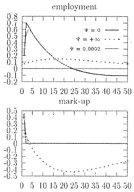
Figure 1: Impulse Response to a Technological Shock (i)
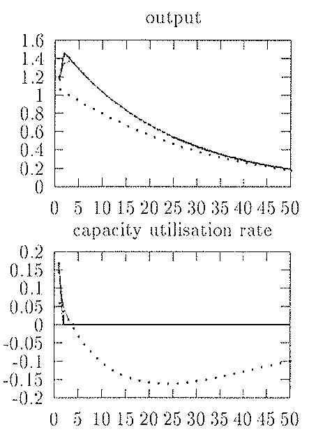
Figure 2: Impulse Response to a Technological Shock (ii)
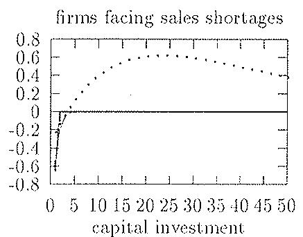
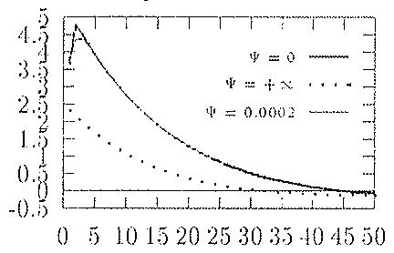
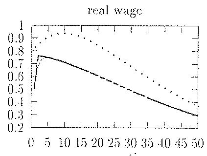
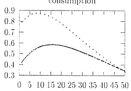
Figure 3: Impulse Response to a Technological Shock (iii)
In Bils and Cho [1994], the capital-labor ratio adjustment cost is written as follows:
\[\mathcal {C} = \gamma k _ {t} \left(\frac {x _ {t} - x _ {t - 1}}{x _ {t - 1}} - \tau\right) ^ {2}\]
where is the steady-state growth rate of the capital-labor ratio x and a scale parameter, the estimation of which is .00969. In our model, the cost function is given by:
\[\mathcal {C} = \frac {\Psi}{2} (x _ {t} - x _ {t - 1}) ^ {2}\]
We set our scale parameter in such a way that the cost of a 1% change in x with respect to its steady state level is identical in the two formulation, given that is null in our model. This gives us the following level of :
\[\Psi = \frac {2 \gamma k}{x ^ {2}}\]
where is the parameter estimated by Bils and Cho [1994] and k,x are the steady state levels of capital and capital-labor ratio in our model.
COLECCION RESUMENES
96-01: "El mercado de depósitos español (1985-1994): Bancos versus Cajas de Ahorro", Juan Coello.
95-01: "Geografía económica y política territorial", CEP, FEDEA (Coordinador), IKEI e IVIE.
TEXTOS EXPRESS
96-01: "La Seguridad Social del siglo XXI y la reforma de las pensiones de 1996", José A. Herce.
95-02: "La reforma de las pensiones: Una encuesta rápida entre los analistas del sistema español",
95-01: "Los problemas de la Sanidad en España: Una encuesta rápida entre los expertos en economía de la salud", Coordinada por José A. Herce, Juan Cabasés y Guillem López i Casasnovas.
DOCUMENTOS DE TRABAJO
96-11: "Idiosyncratic uncertainty, capacity utilization and the business cycle", Jean François Fagnart, Omar Licandro y Franck Portier.
96-10: "La financiación privada de los servicios sanitarios", C. Murillo, S. Calonge e Y. González.
96-09: "Los efectos visibles de la reforma laboral de 1994", Juan F. Jimeno.
96-08: "Diseño y evaluación de estrategias de desregulación en el sector sanitario público en España", Juan Manuel Cabasés Hita y José Martín Martín.
96-07: "Efectos de políticas macroeconómicas en una unión monetaria con distintos grados de rigidez salarial", Carlos de Miguel Palacios y Simón Sosvilla-Rivero.
96-06: "Environmental consequences of the Community Support Framework 1994-1999: Energy consumption and associated emissions in Spain. A HERMIN-model based evaluation", Vicente Antón, Andrés de Bustos, José A. Herce y Simón Sosvilla-Rivero
96-05: "El paro en España: Una encuesta a estudiosos del mercado de trabajo", Sonsoles Castillo, Rosa Duce y Juan F. Jimeno.
96-04: "Los sistemas mixtos de retribución como alternativa al pago por salario y su repercusión sobre la eficiencia del sistema sanitario", Marisol Rodríguez, Diego Rodríguez e Ignacio Abásolo.
96-03: "La creación de un mercado de medicamentos genéricos en España", Félix Lobo.
96-02: "La acreditación de hospitales: Un paso hacia la liberalización del mercado hospitalario español", Lluís Bohigas.
96-01: "La persistencia del paro: Economía y factores institucionales", Juan F. Jimeno.
95-26: "El crecimiento económico en España, 1964-1993: Algunas regularidades empíricas", Oscar Bajo y Simón Sosvilla-Rivero.
95-25: "Análisis de modelos alternativos de retribución de las oficinas de Farmacia", Ramón Gisbert, Joan Rovira y Rafael Illa.
95-24: "Teoría de los ciclos reales y fluctuaciones agregadas de la economía española", Luis A. Puch y Omar Licandro.
95-23: "La financiación hospitalaria basada en la actividad en sistemas sanitarios públicos, resulación de tarifas y eficiencia: El caso de la concertación hospitalaria en Cataluña", Guillem López i Casasnovas y Adam R. Wagstaff.
95-22: "Differential-difference equations in economics: On the numerical solution of vintage capital growth models", Raouf Boucekkine, Omar Licandro y Christopher Paul.
95-21: "Utilización del capital y ciclo económico español", Omar Licandro, Luis A. Puch y Ramón Ruiz-Tamarit.
95-20: "Empleo y sobrecualificación: El caso Español", José García Montalvo.
95-19: "Mecanismos óptimos de adjudicación de contratos públicos: La adquisición de material de telecomunicaciones y la venta del espectro de frecuencias de radio", Alessandro M. Manelli y Daniel R. Vicent.
Este texto se ha extraído automáticamente del documento original. Para citarlo o leerlo con su maquetación, descargue el PDF.
Descargar en PDF