Externalities and Growth in the Spanish Industries* by Berta Moreno Torres**
DOCUMENTO DE TRABAJO 96-17
May, 1996
I want to thank Jose A. Herce, Jeroen Hinloopen, Marion Kohler, Mark Salmon and Robert Waldman for lively discussions and helpful comments. I am also grateful to FEDEA for providing me with some of the data and the bibliography required for the elaboration of this paper. The usual disclaimer applies.
European University Institute Department of Economics Florence. Italy
Index
1. Introduction 2. Literature review 3. Geographical patterns of industrial activity in Spain. 3.1. The data 3.2. Value added and employment 3.3. Payroll and wages 3.4. Specialization and industrial diversity 3.5. Evidence on convergence for the Spanish industries 4. Localization economies 4.1. The modelling 4.2. Empirical evidence 5. Urbanization economies 5.1. The model 5.2. Empirical evidence 6. Conclusions 7. Appendix A 8. Appendix B 9. References
Abstract
Using a panel data set on Spanish regional industries, this paper studies the role of externalities from own industry agglomeration (localization externalities) and from diversification and scale of the local industrial environment (urbanization externalities) for industrial growth. The use of a panel data set allows us to investigate for dynamic and static externalities, while previous work typically relies on cross-sectional data and asserts a role for dynamic effects only. The evidence suggests that both localization and urbanization externalities account for industrial growth. Concerning the time impact of effects, dynamic and static externalities are present, since both past and current conditions affect growth
JEL codes: R11, R30
I. Introduction
In recent years, the study of location problems has attracted considerable attention. No doubt, this increased interest was fostered by the integration of national economies within broader spaces such as the European Union and NAFTA, as well as by their impact on the development of regions and cities. As integration proceeds, regions will compete more intensively to attract industries. Therefore, understanding the determinants of industrial location can help to predict some of the consequences of economic integration.
A potentially important class of localization factors, stressed by the economic geography literature, are agglomeration economies, i.e., the benefits that firms obtain from geographic proximity to one another. There is a long standing debate about whether externalities for a firm derive specifically from other firms in the same local industry or from the general diversity and scale of the local industrial environment . If the former applies, externalities are called (Marshallian) localization economies. They refer to the benefits that firms pertaining to the same local industry get from the formation of pooled labor markets with specific skills, the availability of industry-specific assets and from technological and informational spillovers across firms . On the other hand, if externalities derive from the diversity and the scale of the industrial environment surrounding a given locality, they are generalized external economies or urbanization economies. Urbanization economies are also called Jacobs economies due to Jacobs' (1969) claim that the most important knowledge transfers for firms come from outside the own industry. Additionally, urbanization economies include externalities that derive from the scale of the local industries and can give rise to "thick-market" effects à la Diamond (Diamond, 1982) .
See, for example, Hoover (1948).
This type of benefits were first discussed by Marshall (1890).
Agglomeration economies are extremely appealing because they try to explain simultaneously the location (e.g., city, region or country) in which firms tend to settle and why such locations grow. On the one hand, localization economies imply that industries should specialize geographically to absorb, for instance, knowledge spillovers between firms. Furthermore, regionally specialized industries should grow faster because neighboring firms can learn from each other more easily than geographically isolated firms. On the other hand, urbanization economies predict that industries tend to locate in areas with high industrial diversification and with a large scale of all the industries stimulating knowledge spillovers across industries as well as the local demand and promoting growth.
Recently, a second debate has emerged in the empirical literature on agglomeration economies concerning the question of whether agglomeration economies are mainly static or dynamic . Agglomeration economies are dynamic if the historical industrial environment in a locality (i.e., past agglomeration of the own industry, past diversity and the scale of the local industrial environment in the past) is the relevant aspect to explain the benefits that firms obtain today from geographic proximity. This may occur because the historical industrial environment in a locality means that contemporary firms in that place are able to operate with, e.g., a larger stock of accumulated knowledge and a greater variety of specialized services. Due to the dynamic impact of agglomeration economies, industries will tend to locate and to grow faster in locations where the own industry (all industries in a location) is more represented (more represented and more diverse) historically. Moreover, agglomeration economies are static if the current industrial environment is what matters to explain the contemporaneous benefits that firms enjoy from geographic proximity and as a consequence the pattern of industrial location and growth.
Remark that localization and urbanization economies, despite their apparent contradiction, are not mutually exclusive, the rather offer different views about what is important.
The work of Henderson (1994) constitutes a notable exception.
Empirical studies on agglomeration economies have started to appear recently. Among others, Glaeser et al.(1992), Henderson et al.(1992) and Goicolea et al.(1995) asserted a role for dynamic agglomeration externalities based on comparisons of employment patterns across locations (generally cities) at just two points in time and investigating whether, e.g., past agglomeration and diversity causally affect the current pattern of employment. Dynamic versus static effects were addressed by Henderson (1994) using panel data of county level industrial employment and investigating the explanatory power of the current and the past industrial environment for the growth of local industrial employment. Despite the contribution of the aforementioned papers to clarify the issue of agglomeration economies, two criticism can be made thereof. The first regards the use of labor to measure industrial agglomeration and diversity and to calculate the size and/or the growth of an industry. For labor saving industries this may lead to an underestimation of the presence of those industries in a location and can result in a poor estimation of the growth of the concommitant industries. The second criticism relates to the absence of tests of the congruency of the estimated models; they merely report t-statistics of the parameter estimates, which could be incorrect if the model was misspecified, and measures of the goodness of fit . Thus, the results of the existing literature should be interpreted with considerable reservation until the validity of the estimated models has been tested.
In this paper I investigate the role of localization and urbanization effects as well as of dynamic and static effects for the Spanish industries. To this purpose, I analyze the patterns of industrial activity at the level of the Spanish regions from 1978 to 1991. Key questions to be examined include the following: (1) do industries grow faster in regions where they are more represented?; (2) do regions more industrialized and more diversified industrially benefit from higher labor productivity?, and (3) is there a time pattern of the impact of externalities?
The work of Henderson (1994) constitutes a notable exception.
Formally, my investigation into agglomeration economies is divided into two parts. First, I examine the predictions of localization externalities using a time series of cross sections. Cross sectional units are regional industries (i.e., textiles in Cataluña). In the context of a well specified econometric model, I test empirically whether localization externalities are important for industrial growth by analyzing value added growth as a function of industrial agglomeration in different industries and regions. Second, the test for urbanization economies is performed taking the manufacturing system (i.e., all industries) in a region as the basic unit of analysis. I investigate the determinants of labor productivity in a region, in levels and growth rates, using annual data between 1978 and 1991. The regressors are lagged values of labor productivity, a measure of regional industrial diversity and a measure of the scale of the regional industry. The test for urbanization economies is then performed by analyzing the explanatory power of the latter two variables for labor productivity.
The rest of the paper is divided in four sections. Section II reviews the literature. Section III describes the main variables used in the analysis, namely, value added, labor, agglomeration and diversity, for the Spanish regions. Sections IV an V report the results for localization and urbanization externalities respectively. Finally, section VI presents conclusions.
II. Literature review
Economic geography or spatial economics studies have long been a field of interest for the profession. From a historical perspective, Von Thünen's (1826) study of the pattern of agricultural activities around a city is generally considered as the founder of economic geography. Marshall's (1890) contribution to economic geography is crucial; his analysis of the reasons that explain the geographic concentration of particular industries is still widely used by locational theorists.
During the first half of the 20th century Harris (1954) and Pred (1966) among others emphasized the possibility that economic agglomerations become a self reinforcing process of regions initially more industrialized. They showed that economic agglomerations, by providing a large local market and thus improving firms' market access, are able to attract new industries, which further enlarges their local markets and so on. Such cumulative processes imply that initial advantages (i.e. initial participation of an industry in a region) due to historical accidents may play a major role in explaining the patterns of industrial location and growth. Other economists, namely Christaller (1933), emphasized the trade-off between economies of scale and transportation costs which can result in a hierarchical structure of production sites in which activities with larger scale economies or lower transport costs are concentrated in a smaller number of higher level cities.
One weakness that can be attributed to the geography tradition is its lack of microeconomic foundations and thus the lack of scientific rigor that a theoretical analysis requires. However, the urban economics literature has contributed to overcome that weakness by formalizing the agglomeration economies hypothesis. In a first step, external agglomeration economies were used to explain why only a few cities emerge in an economy. Henderson (1974) was among the first to adopt such an approach, extensively used by the urban economics literature thereafter. He showed that increasing returns external to the firm but internal to the industry and to the city can give rise to agglomeration. Similarly, Fujita (1989) expressed the production function of each firm h in a city as:
\[\mathrm{x} _ {h} = \mathrm{g} (\mathrm{L}) \mathrm{L} _ {h}, \mathrm{g} (\mathrm{L}) > 0 \text { for } \mathrm{L} > 0,\]
where represents the amount of the good produced by firm h when it employs labor and total labor force in the city is L. The function represents the Marshallian external economies that are equally enjoyed by all the firms in the city and tend to generate agglomeration of firms in a city .
The problem with the external economies model of cities put forward above is that it is based on the vague concept of external economies and, when policy recommendations are sought, a more precise specification of the origins of agglomeration economies is needed . This motivated the emergence of a new wave of models where agglomerations economies were modelled endogenously. This new approach, represented by the work of Rivera-Batiz (1988ab), Abdel-Rahman (1988), Fujita (1989) and Abdel-Rahman and Fujita (1990), uses a monopolistic framework to highlight the major forces inducing agglomeration (namely, product and/or input differentiation).
The production aspects of agglomeration were considered by Rivera-Batiz (1988a), Fujita (1989) and Abdel-Rahman and Fujita (1990). They saw the origin of localization economies in the availability of a variety of local (non-traded) producer services . Agglomeration of producers in a city increases the availability of producer services. As a consequence, firms obtain productivity gains, thus providing incentives for producers to migrate to that city. The consumption aspects of agglomeration were studied by, e.g., Hobson (1987) and Abdel-Raman (1988) who showed the utility gains that consumers can obtain by concentrating in space. These include the presence of economies of scale in the provision of local public goods and amenities or the access to a greater variety of local goods and services in larger market areas. Finally, Rivera-Batiz (1988b) developed a model that examines simultaneously the effects of increased diversity in both producer and consumer services on urban agglomeration. In this context, both consumers and producers have an incentive to migrate to the more populated city to benefit from utility gains and productivity gains respectively.
It is assumed that the function is increasing in L, but it may eventually decrease in L: for
for
where is a given constant such that . The first case, where , reflects the positive effects of agglomeration or Marshallian external economies. The second case, where , reflects the negative impact of agglomeration or congestion effects. As long as firms have an incentive to locate in the city.
The reason why the external economies model is so widely used is that external economies are external to individual firms and thus increasing returns to scale become compatible with equilibrium.
The importance of local producer services such as repair and maintenance, legal accounting and consulting, financial and advertising services for industrial agglomeration and regional development is a well documented issue (see, for example, Hansen (1990)).
In urban economics models, the location of cities relative to one another is typically undetermined and the question of how the size of a city affects another city's size is not addressed. These questions, that are crucial from the point of view of regional development, were developed by recent work on regional industrial agglomeration. These models deal with the question of why manufacturing may end up being concentrated in one or a few regions in an economy, giving rise to uneven regional development patterns. One explanation is the existence of urbanization economies at the level of a region, rather than economies specific to a particular industry (i.e., localization economies).
In a simple two-region model, Krugman (1991ab) showed that the existence of urbanization economies may lead to industrialization that becomes a self-reinforcing process of regions with an initial advantage. Urbanization economies emerge from the interaction among transportation costs and economies of scale: consumers have a preference for variety and tend to locate in the location where there are more industrial goods to avoid transport costs while producers are attracted by the concentration of a greater number of consumers. As a consequence, the initial advantage of regions in terms of, e.g., industrial labor endowments may be crucial to determine which region will monopolize industrial activity. An extension of the model to the multi-region case (Krugman, 1992) confirms the relevance of the initial advantage of a region: if a region starts with a large share of workers, it is able to attract more workers, since, as mentioned above, workers will pay fewer transport costs and thus have a higher real income. This stimulates the demand for industrial goods and other firms will tend to locate in that region giving rise to the type of cumulative process already described by Pred (1966). These results, however, were considerably softened by Brackman et al.(1994), who stressed the congestion effects that coincide with the agglomeration of activity in the industrial centre and can explain that small initial regions grow and large initial regions shrink.
Arthur (1990ab) and Arthur, Ermoliev and Kaniovski (1987) presented work which is closely related to the models described above. They saw regional industrialization as a path-dependent process where, in the presence of agglomeration economies, the pattern of regional settlements is determined by the random historical sequence of firms entering the industry and choosing a location. Arthur (1990b) showed that increasing returns to agglomeration, if unbounded, cause concentration of all the industry in a region, and that history, as embodied in the random sequence of arrivals, is all important in selecting which region achieves dominance. Monopoly of industrial activity by a single region, however, can be avoided when there are upper limits to agglomeration benefits.
Finally, there is a related line of work on regional growth that derives uneven growth patterns as a consequence of agglomeration forces. This strand is represented by the work of Engleman and Walz (1995) and Kubo (1995). The former saw the origin of agglomeration economies in the desire of the industrial sector to use a variety of (non-traded) intermediate inputs that are produced by an R&D sector. They show that, at the steady state, the production of intermediate inputs and the production of the industrial good will only occur in the region with the initial advantage in the number of intermediate inputs. The latter did not make any special assumption about the origins of agglomeration economies. Instead, it is assumed that technology is of a fixed coefficient type but there are externalities, in the sense that an accumulation of a region's capital results in reductions in the capital and labor coefficients. As a consequence the pattern of regional industrial development is uneven.
III. Geographical patterns of industrial activity in Spain
3.1 The data
The data set I use for the 17 Spanish regions (Comunidades Autónomas) covers the 14 years between 1978 and 1991. It is constructed from the Encuesta Industrial (Industrial Survey) produced by the Spanish Instituto Nacional de Estadística (National Institute of Statistics).
The Industrial Survey is the major source of statistical information on Spanish industries. The data published by the Industrial Survey is classified by industrial sectors and by regions. The sectorial data provides national totals for the major industrial magnitudes for each of the 89 sectors considered in the Survey. The regional data, on which I concentrate, aggregate the 89 industrial sectors into 18 groups of activity. For each group of activity and each region, the following magnitudes are provided: gross output, value added, number of employees and payroll. I obtain wages by dividing the payroll by the number of employees.
Value added and payroll are transformed into real variables using the industrial price index provided by the Industrial Survey (base 1974=100). The industrial price index from 1978 to 1989 is obtained from Garcia et al(1994). They define the annual index as the average of the monthly figures and change the base of the index from 1974 to 1980. I obtain the 1990-1991 figures from the Industrial Survey and, consistently with Garcia et al., the base is changed from 1974 to 1980.
I have decided to follow a classification of industrial sectors which is in harmony with the European standards, thus facilitating future comparisons with other EU countries. To this end, the data on the 18 industrial sectors recorded by the Industrial Survey are aggregated according to the NACE-CLIO R25 classification which includes 14 sectors. The Industrial Survey, however, considers Agricultural and Industrial Machinery and Office Machinery (NACE-CLIO R25 sectors 6 and 7 respectively) as a single sector. Hence, at the end only 13 industrial sectors are identified. Table 1 below shows the equivalence between both classification systems.
Table 1: Equivalence between the NACE-CLIO R25 and the Industrial Survey industries's classification.
| NACE-CLIO R25 | INDUSTRIAL SURVEY |
| 1. Energy | 1. Energy2. Water |
| 2. Ores and Metals | 3. Metals4. Production and preliminary processing of metals |
| 3. Mineral products | 5. Non-metallic minerals6. Production of non-metallic mineral products |
| 4. Chemical industry | 7. Chemical industry |
| 5. Metal products | 8. Production of metal products |
| 6-7. - Agricultural and indust. machinery- Office machinery | 9. Agriculture, industrial and office machinery |
| 8. Electrical goods | 10. Electrical goods |
| 9. Transportation equipment | 11. Transportation equipment |
| 10. Food, drink and tobacco | 12. Food, drink and tobacco |
| 11. Textile | 13. Textile14. Footwear and leather |
| 12. Paper and printing | 16. Paper, printing and publishing |
| 13. Rubber and plastic | 17. Rubber and plastic |
| 14. Other industries | 15. Timber and furniture18. Other industries |
3.2 Value added and employment
Given the sectorial and a regional perspective, it is not easy to represent in a clear way the variety of data we have. Hence, I have decided to drop the sectorial dimension in this section and to offer a description of the variables for each region at the aggregate industrial level.
The value added series (see Appendix A.1) show quite clearly a declining tendency until, approximately, 1985. This is followed by a recovery of industrial activity that reaches a peak around 1989-1990. Labor employed by the industry typically decreases till 1986 but, contrary to the value added, it continues to decline or remains rather constant in the following years (see Appendix B.1).
The decline of industrial value added and labor until 1985 in most regions provides evidence of the gravity of the Spanish crisis from 1978 to 1985. The industry exhibited a procyclical behaviour, with growth rates below the overall economy's growth rates. At the national level, industrial value added and labor fell at an annual rate of -0.5% and -1.5% from 1978 to 1985, respectively. However, the feature which is most often mentioned to emphasize the strength of the Spanish crisis in the OECD context is the unemployment rate: from 1970 to 1985 this rose from 1.1% to 16%.
During that period, an intense process of structural adjustment took place in the Spanish industry. This development was largely related with the first and second oil shocks, which had serious and long lasting effects on the industry. It should be mentioned that the Spanish industry was extremely dependent on energy consumption compared to the OECD countries. Furthermore, the adjustment to the new situation was somehow delayed by the policy adopted to cope with the shocks . The industry suffered from additional difficulties which derived from its limited technological capacity as well as from its orientation towards the production of goods with newly emerging strong competitors. The unavoidable resulting adjustment process was related to the development of new technologies and materials, to changes in manufacturing demand and, finally, to the marginalization of traditional activities with a strong presence in old areas of industrialization .
After the first oil shock, the reaction of economic authorities was to compensate energy prices by reducing taxes on energetic products. The lack of a decisive intervention of economic authorities results from the priority given to political problems, particularly from 1973 to 1978, while economic problems were marginalized. Only in 1978, after the election of the first democratic government, did energy prices start to increase in line with the international situation.
Around 1985, most of the adjustment had already occurred. As the value added graphs show, the Spanish industry entered a period of intense growth. From 1986 to 1989, industrial growth was enhanced by entrance in the EC and, particularly, by the increase of industrial investments stimulated by the 1992 programme. In 1990, while economic activity tended to stagnate in most industrialized countries, industrial activity achieved a peak. The weakness of the internal demand in 1991 further contributed to the decline of industrial activity in the years following this.
The evolution of regional industrial value added and labor is further illustrated in the graphs 1 and 2. On the horizontal axis, the regions are indicated, while average annual growth rates of value added and labor for 1978/1985, 1986/1991 and 1978/1991 are displayed on the vertical axis. The graphs confirm the divergent behavior of value added and labor from 1986 to 1991 mentioned above. Average annual growth rates of labor are typically small for this period (the national average is 0.35%) and are well below the average value added growth rates (2.1% at the national level).
Graphs 1 and 2 suggest some interesting features regarding the evolution of the distribution of industrial activity across regions. First, the regions more damaged by the crisis are Asturias, Cantabria and País Vasco. Value added and employment grew at a negative rate between 1978 and 1985, while the recovery in the second period is weak and labor continued to fall. These three regions, located on the Cantabric coast, constitute a special case: their industries are largely specialized into basic sectors such as steel, coal and related subsectors (which were particularly hurt by the crisis) and did not tend to diversify over time towards new activities. The high level of environmental pollution in these areas and the absence of a developed service sector related to the industry may also indicate reasons for the industrial decline of this area of old-industrialization .
See, e.g., Sancho and Gradolph (1994) and "El Crecimiento Regional Español ante la Integración Europea" (1990) for detailed discussions of these issues.
Other regions especially damaged by the crisis were those areas which were historically more industrialized and with high industrial densities, namely, Cataluña, Valencia and Madrid. From 1978 to 1985, these regions experienced negative value added and employment growth rates (i.e., -0.6% and -2% respectively) that are below the national average growth rates (i.e., -0.3% and -1.5%). Contrary to the case of the Cantabric regions, both labor and value added tend to recover from 1986.
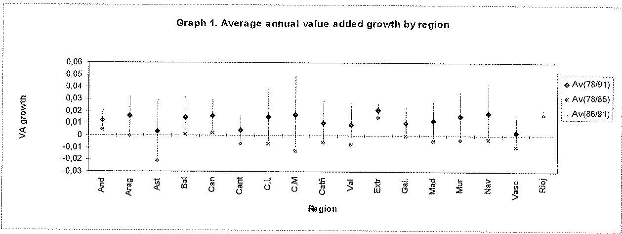
Finally, it is interesting to note the good performance shown, especially after the crisis, by some interior regions, with previously low levels of industrial activity. This applies to Castilla la Mancha, Castilla León, Navarra, Aragón and Extremadura which exhibit annual value added growth rates of 4% from 1985 to 1991. This indicates that industrial activity in Spain is, to a certain extent, subject to a process of dispersion from areas traditionally engaged in manufacturing activity in favor of less industrialized areas.
See, for example, Méndez (1990, p.58) and Velasco (1987, p.23).
No evidence of a persistence of growth rates in regions' value added and employment across subperiods, that is, of positive correlation among growth rates over time was found. The correlation of the growth rate of average value added in each region from 1978 to 1985 with that from 1986 to 1991 is -0.29, meaning that regions more damaged by the crisis do better in the second subperiod. The same thing occurs regarding regional industrial labor (see graph 2), but the correlation of labor growth rates between the two periods is small. Using the data on labor growth for each industrial sector in each region richer information on this issue can be obtained. Moreover, the correlation of the growth rate of employment of each regional industry across the two subperiods is -0.13. Finally, the slope coefficient of a regression of employment growth between 1985 and 1991 on past employment growth (i.e., 1978-1985) and a constant term equals -0.16 (t-value is -1.892) which speaks against the persistence of regional industries' labor growth rates .
3.3 Payroll and wages
At the national industrial level, the participation of payroll in value added increased from 51% in 1972 to 61% in 1975 and started to decline between 1980 and 1982. The rapid increment of payroll relative to value added is not only a consequence of the industrial crisis. Additionally, the dynamics followed by payroll reflects the fragility of the dictatorial government from 1972 as well as the fighting spirit of trade unions. The transition towards democracy, from 1975 onwards, and the consequent legalization of trade unions, it was concluded a period in which the labor market was characterized by the lack of organization of employees, by the strict governmental control of wages negotiations and by the legal difficulties to fire workers.
This stands in sharp contrast with the strong persistence of U.S. states employment growth rates documented by Blanchard and Katz (1992).
The reduction of industrial employment from 1978 to 1985 noted before is partly the result of the cost problems caused by this increase in payroll. Although the largest increments in payroll occurred from 1972 to 1975, the most important employment losses took place from 1981 to 1984, even if the growth of payroll was rather low in this period. However, labor savings were now stimulated by the weakness of industrial demand and were permitted by a more permissive legal regulation of labor firing. The persistent decline of labor after 1986, although at a much lower rate, reflects a further impact of the increase of payroll, namely, the tendency of the industry to change the orientation of production towards labor-saving products. This, in turn, contributed to industrial reconversion .
Wages per worker and the cumulative growth rate of industrial wages across regions between 1978 and 1991 are shown in table 2. At the national level, the growth of industrial wages equals 23% over the whole period (column 3), which corresponds to an annual growth rate of 1.6%. During the industrial crisis (1978-1985), the cumulative and the annual rate of growth of wages (not shown) equal 3% and 0.48% respectively. Not surprisingly, the largest increases occur from 1986 to 1991 when the growth of industrial wages in Spain equals 16% (1.6% per year).
Table 2 shows that the three regions with the poorest performance in terms of labor and value added, namely, Asturias, Cantabria and País Vasco, are those with higher wages per worker in 1991 (see column 2). They all start with wage levels above the national average (column 1). Furthermore, despite the destruction of more than a third of the industrial employment in this area from 1976 to 1991, wages continued to grow at a high rate which, in Cantabria and País Vasco was even above the national average (column 3). Note, however, that these regions were mainly concerned with steel, coal and mining and that they were historically more industrialized. The strength of the trade unions, particularly in these activities can, thus, account for this fact.
See Myro (1989).
Table 2. Wages per employee and growth of wages.
| Region | Wage per worker (mill. ptas) 1978 | Wage per worker (mill. ptas) 1991 | Wage Growth 1991/1978 |
| Extremadura | 0.602 | 1.038 | 0.24 |
| La Rioja | 0.640 | 1.120 | 0.24 |
| Baleares | 0.675 | 1.119 | 0.22 |
| Valencia | 0.693 | 1.102 | 0.20 |
| Murcia | 0.697 | 0.913 | 0.12 |
| Canarias | 0.719 | 1.134 | 0.20 |
| Andalucía | 0.728 | 1.235 | 0.23 |
| C. León | 0.777 | 1.327 | 0.23 |
| Aragón | 0.783 | 1.458 | 0.27 |
| Cataluña | 0.825 | 1.516 | 0.26 |
| Madrid | 0.839 | 1.541 | 0.26 |
| Galicia | 0.927 | 1.494 | 0.21 |
| Cantabria | 0.953 | 1.939 | 0.31 |
| País Vasco | 0.973 | 2.148 | 0.34 |
| C.La Mancha | 0.993 | 1.597 | 0.21 |
| Navarra | 1.030 | 1.724 | 0.22 |
| Asturias | 1.124 | 1.817 | 0.21 |
| Spain | 0.822 | 1.42 | 0.23 |
* Wages are expressed in constant pesetas (1980=100). The first two columns report industrial wages per worker (million pesetas) in 1978 and 1991 respectively. The last column shows the logarithm of wages in 1991 divided by wages in 1978.
There is a remarkable variation of wages per industrial worker across regions (see columns 1 and 2, table 2). The standard deviation of industrial wages across regions is 0.15 in 1978, wages being 27% higher in Asturias (the region with highest wages) than in Extremadura (lowest wage region). Moreover, the standard deviation increases to 0.21 in 1991 and the percentual difference between the higher and the lower region's wages (País Vasco and Murcia respectively) rises to a 37%. This suggests that wages have not converged across regions in the period of our study, an hypothesis that is formally investigated in 3.5.
3.4 Specialization and industrial diversity
The data of the Industrial Survey described in 3.1 allows us to approximate the regional patterns of specialization and diversity of the Spanish industries.
The measure of agglomeration or specialization of a particular industry i in a region j, , is the fraction of the region's value added that this industry represents in that region in a given year, relative to the share of the whole industry in national value added :
\[S _ {k} = \frac {\text { value added of industry i in region j / total value in region j }}{\text { value added of industry in Spain / total value added in Spain }}\tag{1}\]
This variable measures how specialized a region is in an industry, relative to what would be expected if value added in that industry was scattered randomly over all regions. is less than one if the participation of region j in industry i is below the national average, and otherwise it is above one.
In order to measure regional industrial diversity a type of Hirschman-Herfindhal index for value added in a given year is used . For each region, the index is the sum of the squared shares of each industry's value added in total manufacturing value added in the region. That is, if denotes the value added obtained by each industry i in a region j, the index of diversity for region j has the following expression:
This index, defined in terms of industrial labor, was first used by Glaeser et al. (1992) to study geographic concentration in USA.
\[\mathrm{d} _ {j} = \Sigma_ {\forall i} (\mathrm{VA} _ {i j} / \mathrm{VA} _ {j}) ^ {2},\tag{2}\]
where is the sum of value added for all industries in region j. This index measures the lack of diversity in a region. For 13 industrial sectors in our sample, takes a maximum of 1 if value added is concentrated in just 1 industry and a minimum of 0.076 if it is uniformly distributed across all 13 industries .
i'
i'
.
- and thus for all remaining industries .
- and hence for industry and
Minimum diversity occurs if there is a single industrial activity that produces all the value added. Then,
Consequently, the upper bound of the index is one, revealing minimum diversity. Maximum diversity implies that each industry i has an equal participation in manufacturing value added. Then, , being n the total number of industries operating in the region. In this case, equals to 1/n (0.076 in our case where n=13).
Table 3. Industrial specialization and diversity.
| Region | $s_1$ | $s_2$ | $s_3$ | diversity |
| Andalucía | 2.13(10) | 1.74(2) | 1.23(3) | 0.15 |
| Aragón | 1.67(6-7) | 1.5(9) | 1.39(1) | 0.11 |
| Asturias | 7.79(2) | 2.36(1) | 1.15(3) | 0.23 |
| Baleares | 2.88(14) | 2.47(11) | 1.41(3) | 0.18 |
| Canarias | 2.67(10) | 2.04(1) | 1.47(3) | 0.26 |
| Cantabria | 4.14(2) | 1.81(4) | 1.62(5) | 0.12 |
| C. Leon | 2.22(9) | 1.93(13) | 1.84(1) | 0.15 |
| C. Mancha | 1.99(3) | 1.73(1) | 1.34(4) | 0.15 |
| Cataluña | 1.72(11) | 1.64(4) | 1.2(6-7) | 0.101 |
| C. Valencian | 2.27(11) | 2.18(14) | 1.93(3) | 0.11 |
| Extremadura | 3.52(1) | 1.6(10) | 0.71(14) | 0.39 |
| Galicia | 2.25(2) | 1.84(9) | 1.83(1) | 0.14 |
| Madrid | 2.70(8) | 1.76(12) | 1.47(4) | 0.102 |
| Murcia | 6.28(12) | 1.1(1) | 0.95(14) | 0.15 |
| Navarra | 2.81(2) | 1.69(9) | 1.60(8) | 0.103 |
| P. Vasco | 3.99(2) | 2.27(5) | 2.14(13) | 0.107 |
| Rioja | 2.62(10) | 1.6(11) | 1.32(13) | 0.22 |
Table 3 presents evidence on the industrial specialization of the Spanish regions. Industrial agglomeration is approximated by (1) and, for each regional industry, the average value of the index from 1978 to 1991 is reported. In the three first columns of the table, , and show the three largest average values of (1) for each region. The number of the corresponding industrial sectors is in parenthesis beneath these values (see table 1). Partial correlations among , and are weak and do not suggest a relation among the relative specialization of the largest industries in a given region.
Table 3 shows that industrial specialization, in each region, typically involves very different industrial activities. On average, however, energy and water, ores and metals and mineral products (NACE sectors one, two and three, respectively) are the most frequent industrial activities in the ranking of the more specialized regional industries; i.e., they are the first, second or third more agglomerated industries in 39% of cases.
The last column of the table shows the average value of the diversity index (2) from 1978 to 1991. These values suggest that, in general, regions are well diversified . Extremadura is the least industrially diversified region in Spain, being mainly devoted to the production of energy and water . The low level of diversity in Asturias is easily understood given the strong specialization of this region in the production of energy and water, ores and metals and mineral products. La Rioja is a special case: it is a geographically small region, mainly concerned with the production of food and beverages. Not surprisingly, the correlation of the first and fourth columns of table 3 ( and diversity) is 0.32 which means that the agglomeration of the largest industry in a region entails lower industrial diversity.
3.5 Evidence on convergence for the Spanish industries
The foregoing analysis suggests that industrial activity tended to move towards those regions which are less industrialized historically and that the dispersion of regional wages increased over time. The former can imply that there is convergence in industrial activity across regions while the latter suggests that the difference in wages across regions has increased over time. I will now investigate formally the existence of reversion to the mean in the different characteristics of the regions and industries using the following general model of convergence :
See footnote 16.
In Extremadura, energy and water represented 72% of industrial value added in 1991.
\[\begin{array}{r l} & {\log (z _ {k, t + T} / z _ {k, t}) / T = \alpha + \delta l o g (z _ {k, t}) + u _ {k, t},} \\ & {\delta = - (1 - e ^ {- \beta T}) / T,} \end{array}\]
where z is the magnitude of interest in assessing convergence and k=i,j is the index for a regional industry. T is the length of the observation interval, the coefficient is the annual rate of convergence and is a an error term. A between zero and minus one implies reversion to the mean -- e.g., larger initial local industries grow more slowly than smaller ones.
I have applied the basic convergence equation to analyze the behavior of value added, labor wages and agglomeration . In each case, the unit of observation is an industry in a region and hence there are 221 observations. Value added, labor and wages were described in 3.1 and agglomeration is the measure of specialization of a local industry relative to the national total defined in 3.4. Table 4 shows regression estimates of and the implied convergence coefficient, , for 1978 to 1991 and for two subperiods of the sample (1978 to 1985 and 1986 to 1991). The first two columns report the results obtained in a convergence equation that includes a constant term and the log of each regional industry's initial value of the relevant variable. Most of the estimated are significantly negative and hence support the hypothesis of convergence between sectors and regions. The magnitudes, however, vary a great deal across subperiods.
See Barro and Sala-i-Martín (1992).
The limited number of observations for the diversity index (2), i.e., 17 at a given point of time, impeded to investigate the behavior of this variable.
The results for agglomeration show that, in general, industries which were initially less represented in a region have gained relevance. The estimated is negative and significant for the whole sample period, i.e., 1978-91, and for the first subperiod, i.e., 1978-85. These results suggest that, particularly from 1978 to 1985, regions tend to change their specialization and to become more diversified industrially. This can reflect the impact of the industrial crisis which, as mentioned above, affected more dramatically some specialized regions.
Table 4. Convergence across regions and industries: 1978 and 1991.
| Variable | $\delta$ | $\beta (\%)$ | $\delta_R$ | $\beta_R \%$ | $\delta_{R,S}$ | $\beta_{R,S} \%$ |
| VA | ||||||
| 1978-91 | -0.005(-2.502) | 0.52 | -0.008(-2.565) | 0.8 | -0.013(-4.717) | 1.4 |
| 1978-85 | -0.01(-3.28) | 1.1 | -0.014(-3.017) | 1.47 | -0.02(-4.736) | 2.1 |
| 1986-91 | -0.006(-2.507) | 0.61 | -0.009(-2.451) | 0.92 | -0.012(-2.677) | 1.23 |
| Labor | ||||||
| 1978-91 | -0.001(-1.034)) | 0.1 | -0.001(-0.508) | 0.1 | -0.001(-0.489) | 0.1 |
| 1978-85 | -0.003(-1.944) | 0.3 | -0.003(-1.123) | 0.3 | 0.001(0.436) | -0.1 |
| 1986-91 | -0.005(-2.219) | 0.5 | -0.008(-2.428) | 0.81 | -0.01(-4.286) | 1.2 |
| Wages | ||||||
| 1978-91 | 0.001(1.854) | -0.1 | 0.001(1.995) | -0.1 | -0.001(-1.913) | 0.1 |
| 1978-85 | -0.008(-3.454) | 0.82 | -0.009(3.575) | 0.92 | -0.004(-1.893) | 0.41 |
| 1986-91 | -0.002(-0.063) | 0 | 0.003(0.081) | 0 | -0.008(-2.183) | 0.81 |
| Agglomerat. | ||||||
| 1978-91 | -0.005(-2.196) | 0.52 | -0.009(-3.464) | 0.82 | -0.01(-3.186) | 1.07 |
| 1978-85 | -0.017(-4.378) | 1.8 | -0.02(-5.07) | 2.1 | -0.022(-5.159) | 2.38 |
| 1986-91 | -0.002(-0.656) | 0.2 | -0.006(-1.521) | 0.61 | -0.006(-1.448) | 0.61 |
* The table reports the estimates of the convergence equation without dummy variables ( and the implied ), with regional dummies ( , ) and with regional and sectoral dummies( , ). t-statistics are in parenthesis beneath the estimates.
It is interesting to note that the coefficient of the log of past wages for the 1978-1991 is positive. This result argues against convergence of wages of industrial sectors across regions, although the implied is very small. Across subperiods, however, the evidence is mixed; wages tend to converge from 1978 to 1985 but is not significant in the second period.
Columns three and four show the results obtained by estimating the convergence equation with regional dummies (the estimates of the constant term and the regional dummies are not shown to save space). These dummies proxy differences in the steady state values and also absorb fixed regional effects in the error term. The estimates reflects within region convergence between sectors, whereas those from the first two columns are a combination of within and between region and sector convergence. The estimates are generally negative and significant but larger than the estimates without dummies, suggesting that within regions convergence rates across sectors are higher than between regions rates.
The last two columns present estimates of the convergence equation including both regional and sectoral dummies. The main new finding is that the coefficient of is now negative in the wage equation for 1978-1991, suggesting that, holding constant the shocks that affect industrial sectors and regions, wages tend to converge within regions and sectors. Despite this result, the cross-sectional dispersion of the log of wages increased from 1978 to 1991, i.e., there is no convergence in our sample. It appears again that the convergence rates are higher than the rates obtained without dummies or with regional dummies only. Finally, it is interesting to note that the instability of across subperiods persists, despite taking sector and region effects into account.
IV. Localization economies
4.1 The modelling
To test for localization economies, I assume that value added of an industry i in a region j at time t, , , can be written as
\[\mathbf {y} _ {k, t} = \mathrm{g} (\mathbf {l} _ {k, t}) \mathbf {G} (\mathbf {s} _ {k, t}),\tag{1}\]
or, in growth rates,
\[\Delta \mathrm{y} _ {k, t} = \Delta \mathrm{g} (\mathrm{l} _ {k, t}) + \Delta \mathrm{G} (\mathrm{s} _ {k, t}).\tag{2}\]
The first component, , is the technology of the industry which shows the returns of the industry with respect to factor inputs (labor). It can be interpreted as the value added an industry would obtain using a certain amount of inputs in any region. The second component, , is a function of the agglomeration of the own industry, , which captures localization externalities, that is, the externalities related with the size of the own industry. If the hypothesis of localization economies is correct, agglomeration and value added, in levels or in growth rates, should be positively correlated.
The introduction of measures of own industry agglomeration as an explanatory variable in an equation aiming to explain the patterns of industrial location and growth such as (1) and (2) is well justified by theoretical models of agglomeration. It constitutes the basis for some empirical test of agglomeration economies carried out by the literature . The test performed here is based on the same principle --i.e., that agglomeration and value added are positively correlated--, but, additionally, attention is paid to test the specification of the model as well as to the exogeneity of the regressors.
See, e.g., Segal(1975), Glaeser et al(1992) and Henderson et al(1992).
To this purpose, the modelling approach proceeds in two stages. In a first stage, I estimate a vector autoregressive model where no variable is assumed to be weakly exogenous. For each industry i in each region in the sample, the main variables analyzed are the log of value added, , the log of labor inputs, , log of wages, and the log of our measure of own industry agglomeration, . The joint dynamics of the variables is characterized as a vector autoregressive process of order two:
\[\mathrm{X} _ {k} (\mathrm{t}) = \Pi_ {I} \mathrm{X} _ {k} (\mathrm{t-1}) + \Pi_ {2} \mathrm{X} _ {k} (\mathrm{t-2}) + \epsilon_ {k} (\mathrm{t}),\tag{3}\]
where is the vector of observations on the current values of all the variables modelled (i.e., ) and is a vector of random errors assumed to be white noise.
The idea behind the choice of the variables included in the system is the following. First, value added approximates the presence of an industry in a region and helps to measure industrial growth. The value added equation allows us to test for the presence of localization economies and, thus, constitutes the main focus of analysis. The test is performed by estimating the system and investigating the explanatory power of past agglomeration (i.e., and ) in the value added equation. If the estimated coefficient on past agglomeration is significant and positive, the hypothesis of dynamic localization economies is considered to be accepted by the data. Second, labor (number of employees) figures help to determine the returns of the industry with respect to own factors' inputs. Admittedly, capital figures should also be incorporated into the system with that purpose, but the capital figures at the level of regional industries are not available. Third, the inclusion of wages is due to their expected impact on the demand of labor and possibly on value added. That is, it is generally argued that industries tend to move towards low-wage areas and thus wages should be negatively correlated with value added . Additionally, wages tend to be higher in areas where economic activity is more intense and thus represent, to a certain extent, the congestion effects derived from industrial agglomeration. Finally, agglomeration of the own industry takes account of localization effects or Marshallian economies. The measure I use is the index (1) described in 3.4. This measure of agglomeration is constructed using the value added data while the empirical literature generally relies on labor-based agglomeration measures. As mentioned earlier, I also focus on value added instead of labor to approximate industrial growth and analyze the prevalence of localization economies. In this way, I take labor saving industries into account, and avoid the misestimation of growth, agglomeration and the impact of agglomeration for growth for such industries .
See Glaeser et al. (1992).
Estimation of (3) presents the problem that the index of agglomeration is highly correlated over time. That is, the correlation of and is close to one and, thus, a lack of impact of agglomeration on, e.g., value added could be inferred as a result of such a colinearity problem. To deal with this problem, the equations could be first differenced and, since all level variables are in logs, the resulting equations would be in growth rates. This procedure, however, imposes a strong restriction which excludes any impact from past disequilibria in levels. As a consequence, an imperfect test of localization economies would be the outcome. The reason is that the growth rate of the agglomeration index alone is not a suitable approximation for (all) the benefits that firms obtain from geographic proximity. That is, an increase in agglomeration will probably imply an increase in ,e.g., the number of service firms. However, from the point of view of the industry, the relevant thing is the "stock" of service firms and not only the growth in the number of service firms and, of course, this is best represented by the "level" of agglomeration .
To eliminate the colinearity problem while keeping the level of agglomeration, (3) is written in error correction form:
\[\Delta \mathrm{X} _ {k} (\mathrm{t}) = \Gamma_ {J} \Delta \mathrm{X} _ {k} (\mathrm{t-1}) + \Gamma_ {2} \mathrm{X} _ {k} (\mathrm{t-2}) + \epsilon_ {k} (\mathrm{t}),\tag{4}\]
This could be a relevant problem in this work since, as it was shown in section 3.2, industries in our sample tend to save labor.
In general, empirical studies have not taken growth rates of agglomeration externalities variables (see, e.g., Henderson (1994) and Goicolea et al. (1995)).
where , and . In this model, the level of past agglomeration ( ) and the growth rate of agglomeration in the past ( ) in the value added equation, represent the impact of dynamic agglomeration economies.
The first stage comes to an end when tests are conducted to verify whether the system presents any sign of misspecification (e.g., autocorrelation and nonnormality of the residuals) and the results of the tests are satisfactory. Then, in a second stage, I develop a model for value added growth and test the exogeneity of its determinants. If agglomeration is weakly exogenous for the parameters of interest, the test for localization economies is completed by inserting the unlagged agglomeration variable in the model for value added . If the estimated coefficient on the agglomeration variable is positive and significant, the hypothesis of static localization economies (i.e., the impact of (current) growth of agglomeration for (current) value added growth) is considered to be accepted by the data.
The attraction of this modelling approach is that, apart from the choice of variable transformation and linearity for the specified relationship between them, there are no a priori restrictions imposed. Additionally, the hypothesis regarding a priori structure and exogeneity are suitably tested in the context of a well specified system. Finally, the modelling allows us to give evidence on both dynamic and static agglomeration economies while most evidence until now was restricted to dynamic externalities.
The parameters of interest are those relating to labor, wages and agglomeration in the value added equation.
4.2 Empirical evidence
In this section I present the estimated results of equation (4). The analysis is concentrated on the growth of the dependent variables between 1986-1991. Thus, the set of endogenous variables, , is , , and , where the subscript 86-91 indicates that the variable represents the cumulative growth rate between 1986 and . The total number of observations for each variable is 221, corresponding to the 13 industries in the 17 regions in the sample. The regressors are the history of the dependent variables, namely, the lagged value of the dependent variables, , where 78-86 indicates the period 1978-86, and , i.e., the logarithm of the variables in 1978. As it was discussed in section 3, the period that runs from 1978 to 1986 is dominated by a crisis of the industrial system, which can be identified by the declining tendency of both value added and labor series. Industrial activity from 1986 to 1991 experienced high growth rates, partly stimulated by the entrance to the European Community. It is considered that the information contained by the data within these two periods is broadly homogeneous and hence relevant information is not lost by ignoring annual data.
I also include in the regression sectoral and regional indicator variables (listed in appendix B.1), which take the value 1 for all the observations corresponding to a particular region or industrial sector. The reason for the inclusion of these variables is that one can expect to find effects specific to industries or regions in the data set. Regional effects may be present because of unmeasured regional characteristics, such as education, coastal location and land prices. Similarly, sectoral effects are likely to be present due to the omission of variables representing, e.g., market conditions. Actually, the null hypothesis of normality, homoscedasticity and absence of serial correlation was rejected when the system was estimated without these indicators variables, which argues in favor of the existence of sector/region effects.
The parameters of interest are those relating to labor, wages and agglomeration in the value added equation.
The variables are defined in appendix B.1.
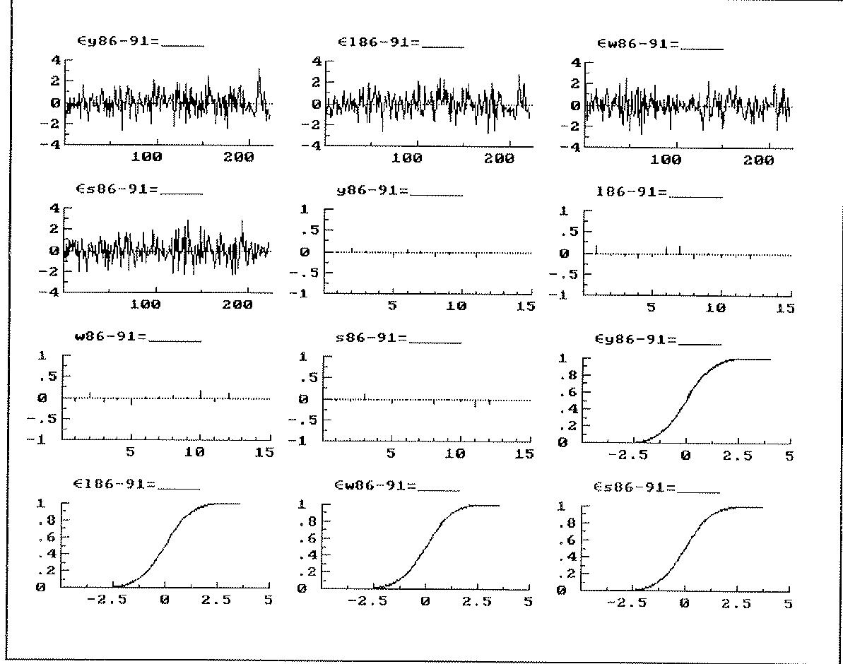
Table 5 reports the OLS estimates for the four equations in the system with 15 indicator variables only: the remaining variables where not significant in the system and the reduction is easily accepted by the overall F-test and reduces the estimation costs. The graphs of the residuals (graph 3) are indicative of a relative random (white noise) appearance: the residuals do not seem to be serially correlated and its standardized cumulative distribution is close to the N(0,1). The diagnostic tests for each single equation and for the system confirm that the residuals are normally distributed and serially uncorrelated. The null hypothesis of homoscedasticity was rejected but standard errors are consistently estimated through a White-type correction of the variance-covariance matrix. The correlation between the actual and fitted values are around 65-80% for value added, labor and wages growth and are lower for the agglomeration equation (45%).
The equation for value added growth (see table 5.A) allows us to get some preliminary results about localization economies. The evidence on the prevalence of dynamic localization economies is partial. That is, the coefficient on past agglomeration ( ) in that equation is statistically significant and positive. This means that regional industries that were more agglomerated in the past (i.e., 1978) have experienced higher value added growth rates between 1986 and 1991, as corresponds to the notion of dynamic localization economies. The growth of the agglomeration index in the past ( ), however, does not have any explanatory power.
Table 5.A. Results for the System. Equation for
| Variable | Coefficient | Std.Error | t-value | t-prob | HCSE |
| $\Delta y_{78-86}$ | -0.24241 | -0.051217 | -4.733 | 0.0000 | 0.044535 |
| $\Delta l_{78-86}$ | 0.11887 | 0.077546 | 1.533 | 0.1269 | 0.10364 |
| $\Delta w_{78-86}$ | 0.31994 | 0.13715 | 2.333 | 0.0207 | 0.14958 |
| $\Delta s_{78-86}$ | -0.038983 | 0.045751 | -0.852 | 0.3952 | 0.054148 |
| $y_{78}$ | -0.27883 | 0.052092 | -5.353 | 0.0000 | 0.046477 |
| $l_{78}$ | 0.21463 | 0.054752 | 3.920 | 0.0001 | 0.051596 |
| $w_{78}$ | -0.0046247 | 0.026543 | -0.174 | 0.8619 | 0.027829 |
| $s_{78}$ | 0.059670 | 0.021632 | 2.758 | 0.0064 | 0.031745 |
| AST | -0.084117 | 0.028930 | -2.908 | 0.0041 | 0.019815 |
| BAL | -0.074299 | 0.032009 | -2.321 | 0.0213 | 0.034129 |
| CAN | -0.12689 | 0.030833 | -4.115 | 0.0001 | 0.035441 |
| CAT | -0.091199 | 0.029564 | -3.085 | 0.0023 | 0.034343 |
| CLE | -0.041169 | 0.028319 | -1.454 | 0.1476 | 0.017505 |
| EXT | -0.12584 | 0.032221 | -3.906 | 0.0001 | 0.038585 |
| ENE | 0.14631 | 0.038954 | 3.756 | 0.0002 | 0.035655 |
| ORE | -0.057907 | 0.030064 | -1.926 | 0.0555 | 0.037596 |
| CHE | 0.020572 | 0.030785 | 0.668 | 0.5048 | 0.033329 |
| MET | -0.10995 | 0.065722 | -1.673 | 0.0959 | 0.067546 |
| MAC | -0.071457 | 0.028557 | -2.502 | 0.0132 | 0.028900 |
| ELE | 0.041620 | 0.027693 | 1.503 | 0.1345 | 0.030599 |
| TRA | 0.10287 | 0.028006 | 3.673 | 0.0003 | 0.031133 |
| FOOD | -0.012407 | 0.031830 | -0.390 | 0.6971 | 0.026774 |
| TEX | -0.14245 | 0.028655 | -4.971 | 0.0000 | 0.032440 |
| Constant | 0.44053 | 0.063939 | 6.890 | 0.0000 | 0.10199 |
RSS Diagnostic tests AR 1-2: F-Form(2, 195) = 0.66871 [0.5135] Normality: [0.5256] Homosc.: F-Form(31, 165) = 2.0393 [0.0023]
Table 5.B. Equation for
| Variable | Coefficient | Std.Error | t-value | t-prob | HCSE |
| $\Delta y_{78-86}$ | 0.039165 | 0.039067 | 1.003 | 0.3173 | 0.048954 |
| $\Delta l_{78-86}$ | -0.20073 | 0.059150 | -3.394 | 0.0008 | 0.078131 |
| $\Delta w_{78-86}$ | 0.13320 | 0.10461 | 1.273 | 0.2044 | 0.11786 |
| $\Delta s_{78-86}$ | -0.018216 | 0.034898 | -0.522 | 0.6023 | 0.045314 |
| $y_{78}$ | -0.023000 | 0.039735 | -0.579 | 0.5634 | 0.039584 |
| $l_{78}$ | -0.039964 | 0.041763 | -0.957 | 0.3398 | 0.040319 |
| $w_{78}$ | -0.016803 | 0.020246 | -0.830 | 0.4076 | 0.021064 |
| $s_{78}$ | 0.025776 | 0.016500 | 1.562 | 0.1198 | 0.023989 |
| AST | -0.069744 | 0.022067 | -3.161 | 0.0018 | 0.019794 |
| BAL | -0.030385 | 0.024416 | -1.244 | 0.2148 | 0.030420 |
| CAN | -0.041969 | 0.023519 | -1.784 | 0.0759 | 0.026758 |
| CAT | 0.11582 | 0.022551 | -5.136 | 0.0000 | 0.023536 |
| CLE | -0.038303 | 0.021601 | -1.773 | 0.0777 | 0.014935 |
| EXT | -0.12163 | 0.024577 | -4.949 | 0.0000 | 0.029042 |
| ENE | -0.054401 | 0.029713 | -1.831 | 0.0686 | 0.030767 |
| ORE | -0.13729 | 0.022932 | -5.987 | 0.0000 | 0.024208 |
| CHE | -0.060979 | 0.023482 | -2.597 | 0.0101 | 0.022302 |
| MET | -0.033600 | 0.050131 | -0.670 | 0.5035 | 0.054138 |
| MAC | -0.030946 | 0.021782 | -1.421 | 0.1570 | 0.023194 |
| ELE | -0.011645 | 0.021124 | -0.551 | 0.5821 | 0.025868 |
| TRA | 0.022393 | 0.021362 | 1.048 | 0.2958 | 0.025415 |
| FOOD | -0.0096431 | 0.024279 | -0.397 | 0.6917 | 0.020622 |
| TEX | -0.083998 | 0.021858 | -3.843 | 0.0002 | 0.026615 |
| Constant | 0.29052 | 0.048771 | 5.957 | 0.0000 | 0.077543 |
RSS Diagnostic tests AR 1-2: F-Form(2, 195) = 2.908 [0.0570] Normality: [0.3942] Homosc: F-Form(31, 165) = 2.0421 [0.0023]
Table 5.C. Equation for
| Variable | Coefficient | Std.Error | t-value | t-prob | HCSE |
| $\Delta y_{78-86}$ | 0.015005 | 0.023045 | 0.651 | 0.5157 | 0.024389 |
| $\Delta l_{78-86}$ | 0.0041918 | 0.034892 | 0.120 | 0.90450 | .036609 |
| $\Delta w_{78-86}$ | -0.63303 | 0.061708 | -10.258 | 0.0000 | 0.077682 |
| $\Delta s_{78-86}$ | 0.023918 | 0.020586 | 1.162 | 0.2467 | 0.021530 |
| $y_{78}$ | 0.051750 | 0.023439 | 2.208 | 0.0284 | 0.022497 |
| $l_{78}$ | -0.044998 | 0.024635 | -1.827 | 0.0693 | 0.023608 |
| $w_{78}$ | -0.0073782 | 0.011943 | -0.618 | 0.5374 | 0.016613 |
| $s_{78}$ | -0.013045 | 0.0097330 | -1.340 | 0.1817 | 0.010296 |
| AS | 0.0040797 | 0.013017 | 0.313 | 0.7543 | 0.011726 |
| BAL | -0.00013710 | 0.014402 | -0.010 | 0.9924 | 0.019300 |
| CAN | -0.035237 | 0.013873 | -2.540 | 0.0119 | 0.016848 |
| CAT | 0.020234 | 0.013302 | 1.521 | 0.1298 | 0.014084 |
| CLE | -0.0075949 | 0.012742 | -0.596 | 0.5518 | 0.007281 |
| EXT | 0.00034244 | 0.014498 | 0.024 | 0.9812 | 0.015125 |
| ENE | 0.044463 | 0.017527 | 2.537 | 0.0120 | 0.019766 |
| ORE | 0.13757 | 0.013527 | 10.170 | 0.0000 | 0.015335 |
| CHE | 0.083409 | 0.013852 | 6.022 | 0.0000 | 0.014086 |
| MET | 0.33715 | 0.029572 | 11.401 | 0.0000 | 0.003504 |
| MAC | 0.025088 | 0.012849 | 1.953 | 0.0523 | 0.011719 |
| ELE | 0.074186 | 0.012461 | 5.954 | 0.0000 | 0.014049 |
| TRA | 0.00094118 | 0.012601 | 0.075 | 0.9405 | 0.014124 |
| FOOD | 0.072394 | 0.014322 | 5.055 | 0.0000 | 0.013607 |
| TEX | 0.0018813 | 0.012893 | 0.146 | 0.8841 | 0.012271 |
| Constant | 0.084287 | 0.028769 | 2.930 | 0.00380 | 0.029882 |
Diagnostic tests AR 1-2: F-Form(2, 195) = 1.6979 [0.1858] Normality: [0.5340] Homosc: F-Form(31, 165) = 2.6285 [0.0000]
Table 5.D. Equation for
| Variable | Coefficient | Std.Error | t-value | t-prob | HCSE |
| $\Delta y_{78-86}$ | -0.12926 | 0.047576 | -2.717 | 0.00720 | 0.047217 |
| $\Delta l_{78-86}$ | 0.13388 | 0.072034 | 1.859 | 0.0646 | 0.070921 |
| $\Delta w_{78-86}$ | 0.24579 | 0.12740 | 1.929 | 0.0551 | 0.13151 |
| $\Delta s_{78-86}$ | -0.050068 | 0.042499 | -1.178 | 0.2402 | 0.047268 |
| $y_{78}$ | -0.10705 | 0.048390 | -2.212 | 0.0281 | 0.059490 |
| $l_{78}$ | 0.10932 | 0.050860 | 2.149 | 0.0328 | 0.060907 |
| $w_{78}$ | 0.015017 | 0.024656 | 0.609 | 0.5432 | 0.028190 |
| $s_{78}$ | -0.011695 | 0.020094 | -0.582 | 0.5612 | 0.020247 |
| AST | -0.043084 | 0.026873 | -1.603 | 0.1105 | 0.019683 |
| BAL | -0.027566 | 0.029734 | -0.927 | 0.3550 | 0.029806 |
| CAN | -0.018862 | 0.028642 | -0.659 | 0.5110 | 0.026967 |
| CAT | -0.032605 | 0.027463 | -1.187 | 0.2366 | 0.031152 |
| CLE | -0.10685 | 0.026306 | -4.062 | 0.0001 | 0.020704 |
| EXT | -0.12341 | 0.029931 | -4.123 | 0.0001 | 0.041822 |
| ENE | 0.090628 | 0.036185 | 2.505 | 0.0131 | 0.038417 |
| ORE | 0.027848 | 0.027927 | 0.997 | 0.3199 | 0.031590 |
| CHE | -0.0074603 | 0.028597 | -0.261 | 0.7945 | 0.036479 |
| MET | -0.064374 | 0.061051 | -1.054 | 0.2930 | 0.064163 |
| MAC | 0.016059 | 0.026527 | 0.605 | 0.5456 | 0.029350 |
| ELE | 0.035999 | 0.025725 | 1.399 | 0.1633 | 0.024972 |
| TRA | -0.016849 | 0.026015 | -0.648 | 0.5180 | 0.029914 |
| FOOD | 0.00057087 | 0.029568 | 0.019 | 0.9846 | 0.023407 |
| TEX | -0.020309 | 0.026619 | -0.763 | 0.4464 | 0.026956 |
| Constant | 0.010347 | 0.059395 | 0.174 | 0.8619 | 0.046749 |
RSS Diagnostic tests AR 1-2: F-Form(2, 195) = 0.50708 [0.6030] Normality: [0.5073] Homosc.: F-Form(31, 165) = 1.2122 [0.2203] Vector tests AR 1-2: F-Form(32, 687) = 1.4577 [0.0509] Normality: [0.0440] Homosc: F-Form(310, 1515) = 1.4653 [0.0000]
Graph 3. System residuals
The equations for value added and labor (table 5.A and 5.B) confirm our previous findings regarding the non-persistence of employment and value added growth rates over time (see section 3.2). The coefficient on in the value added equation is -0.24 (t-value -4.733) and the coefficient on is -0.20 (t-value 3.39) in the labor equation. Accordingly, regional industries with lower value added and labor growth rates between 1978 and 1986 experienced higher growth from 1986 to 1991. Another interesting feature of the value added equation is that the coefficient on past value added ( ) is significantly negative which confirms our previous finding that there has been some convergence in the distribution of industrial activity over the period of our study.
Wage growth between 1978-1986 and 1986-1991 is strongly negatively correlated. The coefficient on in the wage equation is -0.63, indicating that regional industries with higher rates of wage growth in the past experienced lower growth from 1986 to 1991. Moreover, the coefficient on the log of wages in 1978 is not significant so that no evidence is found regarding wage convergence. Finally, it is interesting to note that the coefficient on the log of value added in 1978 is significantly positive, which implies that wages have grown faster in regions where industrial activity was traditionally important.
The last equation of the system, , shows that the rate of growth of industrial agglomeration from 1986 to 1991 is negatively correlated with the rate of growth of value added from 1978 to 1986 and with past industrial value added ( ). The behavior of the agglomeration variable can be explained by the process of adjustment and restructuration of the Spanish industries, which lasted from 1975 to 1985 approximately, and the resulting change in the orientation of production. Thus, it is possible that higher growth of agglomeration between 1986 and 1991 corresponds to regional industries less important traditionally in the concomitant region, which have gained relevance as a consequence of such process.
A model for value added growth was developed by testing whether , and are weakly exogenous for the parameters of interest in the value added equation . A formal test of such hypothesis was performed by estimating and saving the residuals for each equation in the system. The residuals of each equation are called , , and . Moreover, we must reduce and test any overidentifying restrictions. The restrictions imposed are that past wages ( ) did not affect value added growth. Additionally, I impose the restriction that there are no effects specific to the chemical industry and the electrical goods sector.
For a definition of the concept and the tests for weak exogeneity see Doornik and Hendry (1995) and Engle, Hendry and Richard (1983).
Table 6. Model 1. Estimating by FIML. *LR test of overidentifying restrictions [0.0671]
| Variable | Coefficient | Std.Error | t-value | t-prob | HCSE |
| $\Delta y_{78-86}$ | -0.228035 | 0.0926922 | -2.460 | 0.0148 | 0.08059 |
| $\Delta l_{78-86}$ | 0.141174 | 0.160768 | 0.878 | 0.3810 | 0.12269 |
| $\Delta w_{78-86}$ | 0.523854 | 0.283180 | 1.850 | 0.0658 | 0.24415 |
| $\Delta s_{78-86}$ | -0.0324178 | 0.0405520 | -0.799 | 0.4250 | 0.05215 |
| $y_{78}$ | -0.269741 | 0.0759543 | -3.551 | 0.0005 | 0.08105 |
| $l_{78}$ | 0.220070 | 0.0919256 | 2.394 | 0.0176 | 0.078703 |
| $s_{78}$ | 0.0614381 | 0.0198368 | 3.097 | 0.0022 | 0.024347 |
| AST | -0.0547291 | 0.0360502 | -1.518 | 0.1306 | 0.04260 |
| BAL | -0.0583235 | 0.0261115 | -2.234 | 0.0266 | 0.031052 |
| CAN | -0.0928165 | 0.0341701 | -2.716 | 0.0072 | 0.036042 |
| CAT | -0.0588459 | 0.0524089 | -1.123 | 0.2629 | 0.055524 |
| CLE | 0.000985339 | 0.0531825 | 0.019 | 0.9852 | 0.058010 |
| EXT | -0.0589792 | 0.0672686 | -0.877 | 0.3817 | 0.085272 |
| ENER | 0.117546 | 0.0638387 | 1.841 | 0.0671 | 0.059198 |
| ORE | -0.0913918 | 0.0475380 | -1.922 | 0.0560 | 0.043925 |
| META | -0.246458 | 0.133109 | -1.852 | 0.0656 | 0.10976 |
| MAC | -0.0786465 | 0.0231602 | -3.396 | 0.0008 | 0.016305 |
| TRA | 0.100195 | 0.0237532 | 4.218 | 0.0000 | 0.021802 |
| FOOD | -0.0446890 | 0.0282072 | -1.584 | 0.1148 | 0.022330 |
| TEX | -0.113666 | 0.0428123 | -2.655 | 0.0086 | 0.043361 |
| $R\Delta l_{86-91}$ | 0.310681 | 0.514340 | 0.604 | 0.5465 | 0.42082 |
| $R\Delta w_{86-91}$ | -0.394466 | 0.376283 | -1.048 | 0.2958 | 0.321511 |
| $R\Delta s_{86-91}$ | 0.240861 | 0.549330 | 0.438 | 0.6615 | 0.532064 |
| $\Delta l_{86-91}$ | 0.291704 | 0.510074 | 0.572 | 0.5681 | 0.429555 |
| $\Delta w_{86-91}$ | 0.482765 | 0.361942 | 1.334 | 0.1838 | 0.310765 |
| $\Delta s_{78-91}$ | 0.255622 | 0.546649 | 0.468 | 0.6406 | 0.508330 |
| Constant | 0.312449 | 0.178498 | 1.750 | 0.0816 | 0.16062 |
Since the restrictions imposed were not rejected by the likelihood ratio test, the unlagged explanatory variables and the residuals from the respective equations were inserted into the value added growth equation. The FIML estimates, presented in table 6, show that the estimated coefficients for the residuals are not significant. Hence, the hypothesis that labor, wages and agglomeration are weakly exogenous, can be accepted. This suggests that the marginal process for labor, wages and agglomeration can be left unmodelled when value added growth is studied.
Table 7. Model 2: Value added growth between 1986-91.
| Variable | Coefficient | Std.Error | t-value | t-prob | HCSE |
| Constant | 0.28703 | 0.036274 | 7.913 | 0.000 | 0.05411 |
| $\Delta l_{86-91}$ | 0.57702 | 0.053679 | 10.749 | 0.0000 | 0.068332 |
| $\Delta s_{86-91}$ | 0.51976 | 0.050412 | 10.310 | 0.000 | 0.060566 |
| $\Delta y_{78-86}$ | -0.16335 | 0.028169 | -5.799 | 0.0000 | 0.028550 |
| $\Delta l_{78-86}$ | 0.14845 | 0.048116 | 3.085 | 0.0023 | 0.062990 |
| $y_{78}$ | -0.14857 | 0.024288 | -6.117 | 0.0000 | 0.027720 |
| $l_{78}$ | 0.11522 | 0.025478 | 4.522 | 0.0000 | 0.028475 |
| $s_{78}$ | 0.043125 | 0.013164 | 3.276 | 0.0012 | 0.019889 |
| BAL | -0.040076 | 0.019249 | -2.082 | 0.0386 | 0.016752 |
| CAN | -0.085332 | 0.018902 | -4.515 | 0.0000 | 0.018625 |
| CLE | 0.037340 | 0.018742 | 1.992 | 0.0477 | 0.010878 |
| ENE | 0.086711 | 0.021007 | 4.128 | 0.0001 | 0.027061 |
| MAC | -0.064233 | 0.016320 | -3.936 | 0.0001 | 0.011080 |
| TRA | 0.092500 | 0.016786 | 5.511 | 0.0000 | 0.017198 |
| TEX | -0.080475 | 0.017294 | -4.653 | 0.0000 | 0.015046 |
* The regression uses FIML to estimate the equation. ***Diagnostic tests AR 1-2: F-Form(2, 204) = 2.5694 [0.0791] Normality: [0.1386] Homosc: F-Form(21, 184) = 2.8661 [0.0001] Functional form: F(1,205) = 0.30706 [0.5801]
Model 2, a parsimonious reduction of model 1 where all variables are significant is our selected model. The results, displayed in table 7, show that the coefficient on the log of past agglomeration is positive, as was noted above for the value added equation in the system, indicating that industries grow faster in regions where they are historically more represented. The (positive) direct impact that conditions of 1978 have on growth in 1986-91 suggests the presence of dynamic externalities of a Marshall-type that can be related to the presence of an ageing, maturing or transmission mechanism (i.e., about technology, suppliers, etc.). Model 2 shows that industries benefit also from increased concentration of the own industry. That is, the coefficient on is positive and statistically significant, which can be taken as indicative of the existence of static localization effects.
It is interesting to note that past agglomeration was not significant in the labor equation of the system: the coefficients of both and are insignificant. Regression results (not reported), show that agglomeration is weakly exogenous for the parameters of interest in the labor equation and that the unlagged agglomeration variable is insignificant. In conclusion, agglomeration has a very different impact for value added and for labor and thus the question of whether it is labor or value added that is the relevant variable to analyze localization economies becomes decisive. I hypothesized that the relevant variable is value added and not labor. Beyond the aforementioned problem concerning labor-saving industries, it should be stressed that the primitive concept of localization economies is such that firms obtain productivity gains from geographic proximity for a given amount of inputs. Thus, not denying the possibility that localization economies can stimulate labor demand, for the purpose of testing I find value added more reliable than labor.
Surprisingly, wages are not significant in model 2 even if higher levels of value added in the past ( ) led to higher rates of growth of wages in 1986-1991. One would then expect that industries tend to reallocate towards lower wage areas. The evidence, however, suggests that labor-cost conditions are not crucial for the location decision of firms. Regression results (not reported) revealed that the contemporaneous growth of wages is an influential factor in explaining growth of labor in 1986-1991. That is, the coefficient on in the labor equation is significant and negative, which suggests the existence of an immediate response to the change in wages whereby firms react to, e.g., an increase in wages by hiring fewer workers. However, past wages are not significant and hence the hypothesis that there is a lagged response (adjustment) to wage conditions is rejected. The absence of a dynamic response of labor to wages is somewhat surprising since it can be expected that firms react to wage conditions with a certain delay. That is, part of the response to changes in effective wages is to adjust capital-labor ratios, which is delayed by capital investments and technology turnover. Moreover, responses to changes in local wages are delayed by union contracts which fix wages facing firms within the own industry for a discrete time period. Thus, for heavily unionized industries, effective wages do not respond to changes in the current wage in a region. The response comes when contracts are renegotiated and thus a firm's effective wages may be based on a contract negotiated some years ago, and those negotiations will have been based on local wage conditions for the several years prior to that time. As a consequence, one could expect that past wages have an impact on labor demand but this hypothesis is not accepted by our data.
V. Urbanization economies
5.1 The model
Urbanization effects emerge at the level of a given geographic area and thus are likely to have an impact over all industries located in that region. Accordingly, I take regions as the basic unit of analysis and the test for urbanization economies is performed by analyzing the role of regional diversity and scale in explaining labor productivity across regions. Moreover, I hypothesized that labor productivity can be written as:
\[Y _ {j, t ^ {-}} \propto Y _ {j, t - 1 ^ {+}} \sum_ {p - 1} ^ {q} \beta_ {p} d _ {j, t - p ^ {+}} \sum_ {p = 1} ^ {q} \delta_ {p} S C _ {j, t - p ^ {+}} \in_ {j, t ^ {p}}\tag{5}\]
where denotes the logarithm of labor productivity and j and t index region and time respectively. and are the logarithm of our measures of regional industrial diversity and scale which capture urbanization externalities. Diversity is the Hirshman-Herfindhal index defined in 3.4, and scale is approximated as the participation of a region in the national industry. It is assumed that
\[\mathrm{E} [ \mathrm{d} _ {j, t}, \epsilon_ {j, t + s} ] = \mathrm{E} [ \mathrm{SC} _ {j, t}, \epsilon_ {j, t + s} ] = 0, \forall s > 0.\]
Hence, equation (5) implies that there are no strictly exogenous variables but merely predetermined ones.
If greater diversity enhances productivity, an increase in the measure of regional diversity, the Hirshman-Herfindhal index , will decrease productivity and thus the estimated coefficients for the lagged diversity variables are expected to be negative . If a large scale of the industry means that firms benefit from, e.g., more specialized service or intermediate inputs and obtain productivity gains, the coefficients for the scale of the industry should be positive. Additionally, allowing for a lag structure to the regional externality variables implies that one can discern whether the historical or just the current industrial environment is important. The lag structure is hypothesized to start at t-1 and is allowed to run q periods. Following Henderson (1994), I assume that t-1 corresponds to a context where firms' decisions in period t are based on the best information about current production conditions, which are previous periods' realizations. Similarly, and capture the benefits that firms obtain in period t as a result of the current industrial environment and thus are indicative of static urbanization effects. Values for represent a role for history, where prior realizations contribute to the current environment for production (i.e., dynamic effects).
The problem with estimating (5) is that diversity and scale measures are highly correlated over time. To solve this problem, (5) is reparameterized as follows
\[Y _ {j, t} = \alpha Y _ {j, t - 1} + \sum_ {p - 1} ^ {q - 1} \beta * _ {p} \Delta d _ {j, t - p} + \beta * _ {q} d _ {j, t - q} + \sum_ {p - 1} ^ {q - 1} \delta * _ {p} \Delta S C _ {j, t - p} + \delta * _ {q} S C _ {j, t - q} + \epsilon_ {j, t},\tag{8}\]
\[\beta_ {p} ^ {*} = \sum_ {i = 1} ^ {p} \beta_ {t - i}, \quad \beta_ {q} ^ {*} = \sum_ {i = 1} ^ {q} \beta_ {t - i}, \quad \Delta d _ {j, t - p} = (d _ {j, t - p} - d _ {j, t - p - 1}),\]
Remember that the index of diversity measures lack of diversity.
This reparameterization is without loss of generality and involves no loss of information. Since the variables are defined in logs, this specification sets labor productivity in a given region as a function of past labor productivity, the growth of regional diversity and scale and the level of these variables in the past (i.e., at t-q).
The econometric set up used for the estimations is the fixed/random effect model. This model imposes constant slope coefficients across units assuming that differences across units can be captured in the constant term. The constant term includes relatively time invariant unmeasured regional attributes. The latter would include the notion of local culture affecting the local, legal, business and institutional climate as well as differences in unmeasured resources. In the case of fixed effects the slope coefficient and the (regional) effects can be estimated consistently and efficiently by OLS after the data are transformed by subtracting group means from each observation (within-group estimators). The random effects model views individual specific constant terms as randomly distributed across units. The constant term for each unit, , is expressed as
\[\mathrm{a} _ {\mathrm{j}} = \mathrm{a} + \mathrm{u} _ {\mathrm{j}}, \text { for all } j,\]
where is the random disturbance characterizing the jth unit (constant through time) and it is assumed that
\[\begin{array}{l} \mathrm {E[ \epsilon_ {jt} ] = E[u_ {j} ] = 0 ,} \\ \mathrm {E[ \epsilon_ {jt} ^ {2} ] = \sigma_ {\epsilon} ^ {2} ,} \\ \mathrm {E[u_ {j} ^ {2} ] = \sigma_ {u} ^ {2} ,} \\ \mathrm {E[u_ {j} \epsilon_ {it} ] = 0 \quad for all i,j and t ,} \\ \mathrm {E[ \epsilon_ {jt} \epsilon_ {is} ] = 0 if j\neq i or t\neq s ,} \\ \mathrm {E[u_ {j} u_ {i} ] = 0 if j\neq i .} \end{array}\]
In the case of random effects, GLS is the appropriate estimator (since in general). The Hausman test is used to discriminate among fixed and random effect .
5.2. Empirical Evidence
Table 8 presents the estimation results of (6), obtained using annual data on labor productivity, regional diversity and scale for the Spanish regions/industries from 1978 to 1991 . In terms of the lag structure, q is set at 3, i.e., I look back four years from the current point in time. This implies that, using a fourteen year panel, in estimation of (6) eleven years (14-q=11) are covered. As it will be discussed later, I found that expanding q beyond 3 does not provide much information since most effects tend to peak at t-1 and disappear at t-3.
Since the null hypothesis that there are random effects was rejected by the Hausman test, I report only the results corresponding to the fixed effects model. Table 8 shows that the coefficient on and are negative and statistically significant, arguing in favor of the presence of across industries externalities. On the other hand, the coefficient on the log of diversity in is statistically insignificant. In conclusion, diversity of the local industrial environment seems to be a relevant source of spillovers but it achieves a peak just at ; then the effect diminishes at so that at it has a small and insignificant coefficient. The impact of regional diversity, thus, is mainly static; the dynamic influence is rather limited.
The Hausman test is based on the fact that the random effect approach treats the individual effects as uncorrelated with other regressors, while the fixed effects approach does not make such an assumption. The null hypothesis is that is that individual effects are indeed uncorrelated with other regressors. Thus, if the null is accepted, the hypothesis of random effects cannot be rejected.
The variables are defined in appendix B.2
Table 8. Regional labor productivity
| Variable | Coefficient | Std. Error | t-ratio | Prob|t|≥x |
| Yj,t-1 | 1.0286 | 0.08101 | 12.697 | 0.00000 |
| $\Delta d_{j,t-1}$ | -0.33515 | 0.08047 | -4.165 | 0.00005 |
| $\Delta d_{j,t-2}$ | -0.16951 | 0.08229 | -2.060 | 0.04086 |
| $d_{j,t-3}$ | -0.01709 | 0.02894 | -0.591 | 0.55556 |
| $\Delta SC_{j,t-1}$ | 1.6661 | 0.1596 | 10.442 | 0.00000 |
| $\Delta SC_{j,t-2}$ | 1.0629 | 0.1812 | 5.866 | 0.00000 |
| $Scj,T--3$ | -0.00409 | 0.01443 | -0.284 | 0.77703 |
* Random vs Fixed (Hausman) = 0.0001[0.999] DW=1.98 Normality = 1.1116[0.5736]
The scale of a regional industry has a positive impact on labor productivity in a region; the coefficients on and are significant and positive, meaning that labor productivity is higher in regions that experienced higher growth rates of its industrial scale in the last years. The evidence reveals that the impact of the scale of the regional industry is not very persistent: the coefficient of is insignificant suggesting that the positive effects of the scale tend to evaporate beyond q=3.
The externality variables should also have an impact on the growth rate of labor productivity. That is, value added per worker should be higher in regions with a larger scale of the industry and more diversified because this facilitates, e.g., communications and information spillovers among regional industries and firms benefit from a larger quantity of specialized service firms. This, in turn, attracts other firms to that region stimulating further spillovers and productivity gains. To investigate the influence of the industrial environment on the growth of labor productivity, equation (5) is first differenced:
\[\Delta Y _ {j, t} = \alpha \Delta Y _ {j - 1} + \sum_ {P - 1} ^ {\sigma} \beta_ {P} \Delta d _ {j, t - p} + \sum_ {P - 1} ^ {\sigma} \delta_ {p} \Delta S C _ {j, t - p} + \Delta \epsilon_ {j, t}\tag{7}\]
Since all variables are defined in logs, equation (7) is in growth rates, relating growth of labor productivity in a region to its lagged value and to the growth of diversity and scale.
Table 9. Growth of labor productivity
| Variable | Coefficient | Std. Error | t-ratio | Prob|t|=x |
| $\Delta Y_{j,t-1}$ | 0.15135 | 0.0785 | 1.927 | 0.05569 |
| $\Delta d_{j,t-1}$ | -0.15317 | 0.0695 | -2.513 | 0.15543 |
| $\Delta d_{j,t-2}$ | -0.21627 | 0.0893 | -2.419 | 0.01667 |
| $\Delta d_{j,t-3}$ | -0.03083 | 0.0854 | -0.361 | 0.71872 |
| $\Delta SC_{j,t-1}$ | 1.8495 | 0.2315 | 7.989 | 0.00000 |
| $\Delta SC_{j,t-2}$ | 1.0865 | 0.2343 | 4.637 | 0.00001 |
| $\Delta SC_{j,t-3}$ | 0.6057 | 0.2248 | 2.695 | 0.00778 |
* Random vs. Fixed Effects (Hausman) = 0.00010[0.999] Normality:
The estimation results of equation (7) are reported in table 9. There is an initial diversity effect, where a 1% increase in the last year diversity (i.e., a 1% decrease of the HHI, ) increases labor productivity in the region today by 15%. It is interesting to note that direct effects from two years ago are stronger: the coefficient on is statistically significant and its absolute value is larger in magnitude than the coefficient on . As before, the change of diversity at q=3 is not significant. On the other hand, scale effects are stronger and more persistent in the growth equation than in the level equation. The coefficients on are all statistically significant and positive arguing in favor of the existence of scale effects.
I have estimated equations (6) and (7) with q=4,5. The passage to q=6 implies too few degrees of freedom to draw any sensible conclusions. Estimation results (not reported) show that extending the lag structure beyond q=3 does not change sensibly our prior results concerning diversity and that the coefficients on diversity become insignificant beyond q=2. These results for industrial diversity are somewhat surprising since one would expect that when an increase in local diversity improves the stock of knowledge there is a diffusion process where it takes time for knowledge to spread and a maturing process where firms want to observe if the new information is good. The results, however, mainly speak of a static impact of diversity. As regard the role of the industrial scale in a region, the most remarkable feature observed is that the increase of the scale at time t-4 and t-5 is still positive and significant (although smaller in magnitude) in equation (7).
VI. Conclusions
During the 80s Spanish industries experienced an important process of adjustment stimulated by a new international situation resulting from the oil shocks and by a new internal environment marked by political and economic liberalization. During this period, the geography of industrial activity went through some related transformations. Moreover, there was a decline of the well known tendency which during the 60s and the 70s indicated the polarization of activity around the areas of traditional industrialization, namely, Cataluña, Madrid and the Cantabric coast. The results presented above shows that the distribution of value added across regions and sectors tend to become more even from 1978 to 1991. This study also suggests a change in the pattern of specialization of regional industries, which probably is due the industrial crisis and a tendency, at least for some regions, to become industrially more diversified.
The basic objective of this work, however, has not been to analyze the changes in the geography of production, a subject which has already been
extensively treated. Instead, I have used recent models of economic geography and agglomeration economies as a guide to highlight some empirical regularities that assist in understanding the reasons for industrial growth across the Spanish regions between 1978 and 1991. The main contribution of this paper is to analyze the dynamic and static influence of the territory as a source of externalities. While the other empirical literature typically concentrates on cities, this work takes regions as the basic geographic area allowing us to investigate the empirical relevance of agglomeration externalities at the level of broader areas. The results presented suggest that, in order to maintain strength in a particular industry, a region needs a degree of agglomeration in that industry. Furthermore, it also needs a surrounding diverse and large manufacturing system.
The results for localization economies show that agglomeration of an industry in the past supports growth. This finding is considered as evidence of dynamic effects which reflect the presence of an ageing, maturing mechanism. Additionally, contemporaneous changes in agglomeration are positively related to the growth of an industry and thus we also find evidence of static effects. In conclusion, the Marshallian model developed in the urban economics literature seems to be generally consistent with the evidence presented here.
I also find evidence in favor of the prevalence of urbanization effects related to the industrial environment that surrounds a regional industry. Labor productivity is higher in regions that evolve towards a more diversified industrial structure, supporting Jacob's (1969) hypothesis of across industries knowledge spillovers. Additionally, the growth of the scale of the manufacturing system in a region is positively correlated with labor productivity, indicating the presence of the type of regional externalities put forward by Krugman (1991ab, 1992). Regarding the time impact of the effects, lagged responses to the industrial environment variables have a large initial impact at q=2 which rapidly become smaller and statistically insignificant. The scale of a regional industry tends to have a more persistent impact than industrial diversity on labor productivity: for the growth equation significant effects persist through the maximum length of the lag structure considered, q=5, or six years ago.
Thus the evidence suggests that there are net benefits for firms to locate in areas of high industrial activity and to interact with firms pertaining to different industries. The growth of regions is one manifestation of this phenomenon. The results would imply, for example, that open societies, with substantial labor mobility across industries and within industries as well as with an open immigration policy, will exhibit a greater spread of ideas and growth. Also, it would argue in favor of the concentration of activity in a fixed number of hours per day, i.e., to limiting opening hours, in order to have more agents operating together at the same time thus facilitating spillovers.
Appendix A. Industrial Value Added and Labor per Region
A.1. Industrial Value Added per Region (million pesetas 1980)
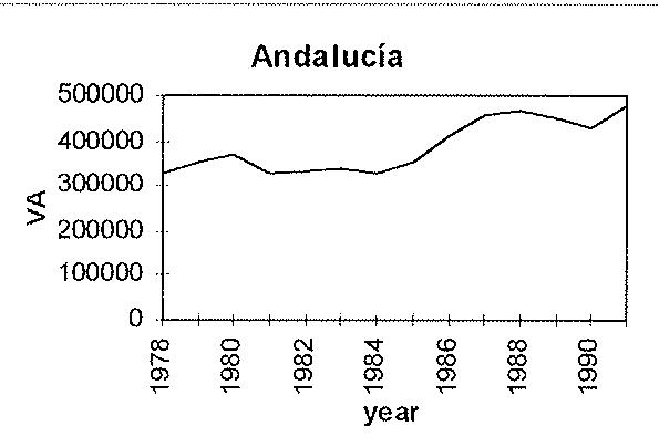
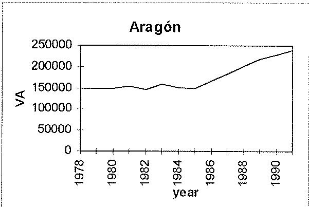
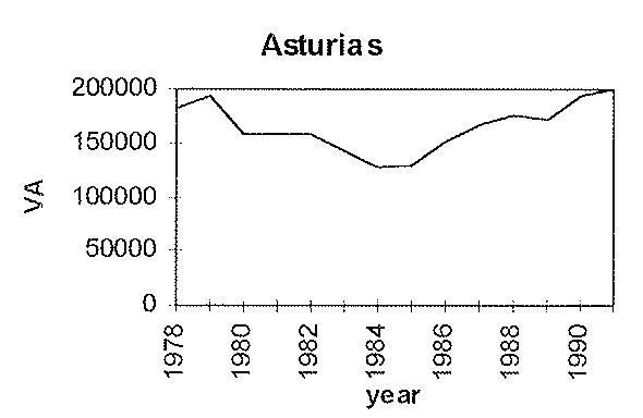
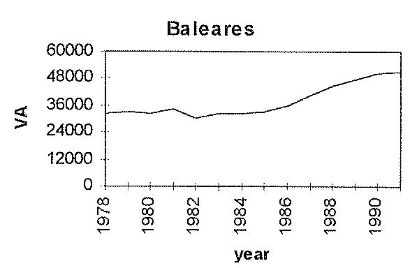
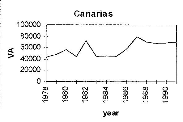
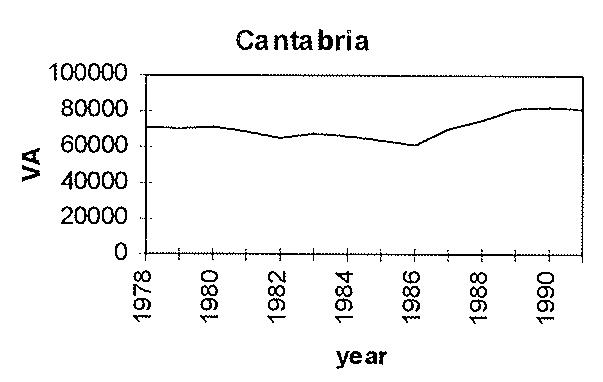
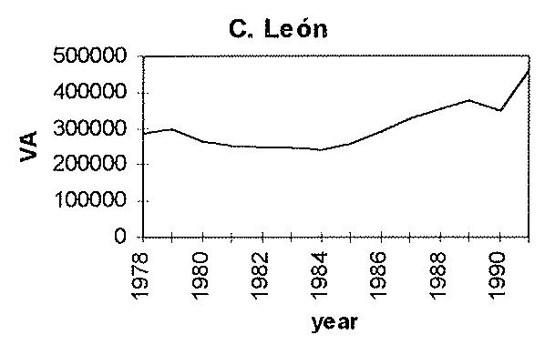
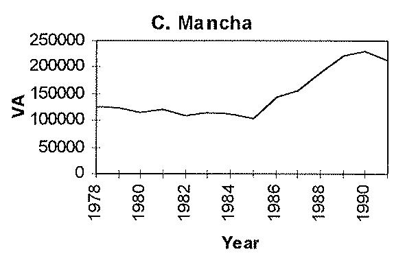
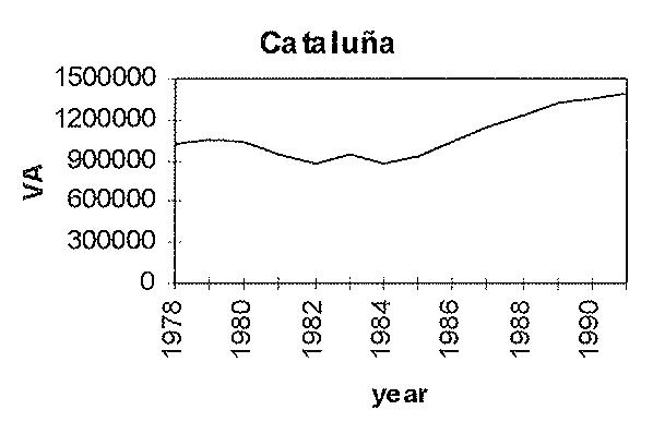
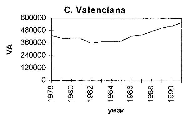
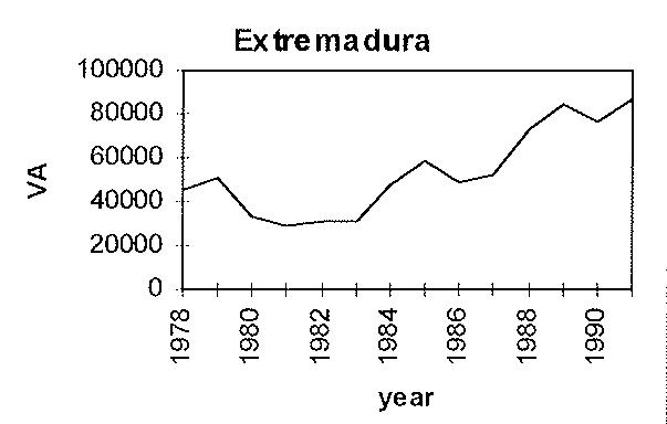
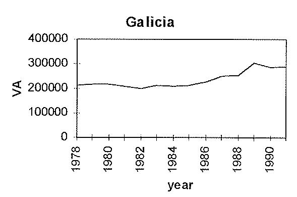
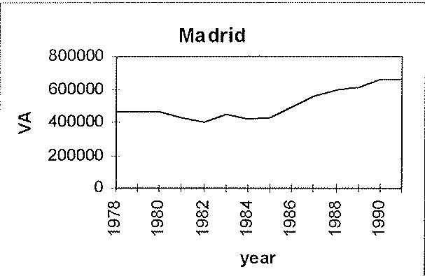
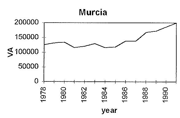
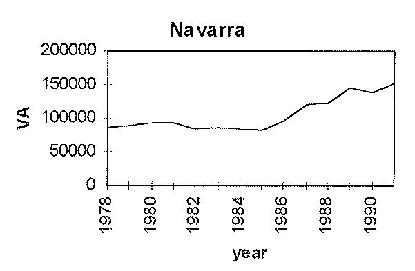
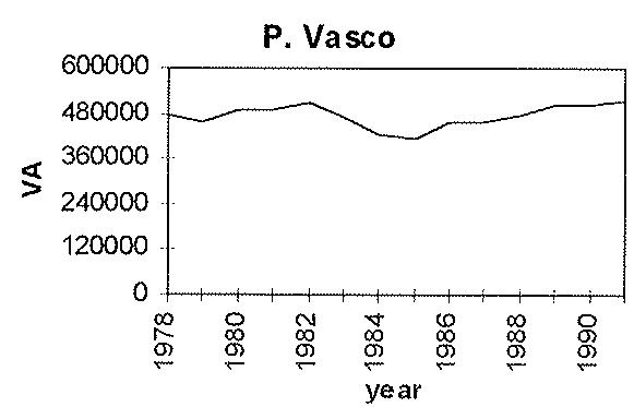
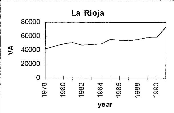
APPENDIX B
B.1. List of variables in tables 5-7
The sample unit is an industry in a region. The total number of observations in a given point of time is 221 (13 NACE industries in 17 regions). Growth rates are defined as the logarithm of a variable at time t divided by the variable in t-1.
Growth rate of value added of an industry in a given region from 1986 to 1991. Value added is defined in million pesetas (constant pesetas 1980=100).
Cumulative growth rate of value added of an industry in a given region from 1978 to 1986.
Logarithm of value added in 1978
Growth rate of labor (i.e., number of employees) from 1986 to 1991
Growth rate of labor from 1978 to 1986.
Logarithm of labor in 1978
Growth rate of wages from 1986 to 1991. Wages are expressed in million pesetas (constant pesetas ).
Growth rate of wages from 1978 to 1986.
Logarithm of wages in 1978 Growth rate of the agglomeration index from 1986 to 1991. The measure of agglomeration was defined in section 3.4 (Index (1)).
Growth rate of agglomeration from 1978 to 1986.
Logarithm of wages in 1978
The variables listed below are indicator variables, for regions and industrial sectors. For example, the regional dummy AND takes the value 1 for all the industries in Andalucía and zero otherwise.
| Variable | Region | Variable | Sector |
| AND | Andalucía | ENE | Energy |
| ARG | Aragón | ORE | Ores and Metals |
| AST | Asturias | MIN | Mineral products |
| BAL | Baleares | CHE | Chemical ind. |
| CAN | Canarias | MET | Metal Products |
| CAT | Cantabria | MAC | Machinery |
| CLE | C. León | ELE | Electrical goods |
| CMA | C. Mancha | TRA | Transport. equ. |
| CAÑ | Cataluña | FOOD | Food,drink&tob |
| CVA | C. Valenciana | TEX | Textile |
| EXT | Extremadura | PAP | Paper and print. |
| GAL | Galicia | RUB | Rubber&plastic |
| MAD | Madrid | OTH | Other industries |
| MUR | Murcia | ||
| NAV | Navara | ||
| PVA | País Vasco | ||
| RIO | La Rioja |
B.2. Definition of variables in tables 8-9
The sample unit are regions. The total number of data points are 14 years for each region before differencing. Annual growth rates are defined as the logarithm of a variable at time t divided by the variable at t-1.
Yj,t-p Logarithm of labor productivity in a region at t-p. Labor productivity equals industrial value added (million pesetas 1980) divided by industrial labor (number of employees).
Annual growth rate of labor productivity in a region.
Logarithm of regional industrial diversity. Diversity is defined as:
\[\mathrm{d} _ {j} = \sum_ {\forall i} (\mathrm{VA} _ {i j} / \mathrm{VA} _ {j}) ^ {2},\]
where denotes the value added obtained by each industry i in theregion and is the sum of value added for all industries in the region
Annual growth rate of regional diversity.
Scj,tp Logarithm of the scale of the industry in a region. The scale is approximated by the participation of a regional industry relative to the national industry. That is,
\[\mathrm{SC} _ {\mathrm{j}} = \left(\mathrm{VA} _ {j} / \mathrm{VA} _ {N}\right),\]
where equals industrial value added in Spain at a given point of time.
Annual growth rate of regional scale.
References
- Abdel-Rahman, H (1988). "Product Differentiation, Monopolistic Competition and City Size". Regional Science and Urban Economics 18.
Abdel-Rahman, H and M. Fujita (1990). "Product Variety, Marshallian Externalities and City Sizes, Journal of Regional Science No. 30.
- Arthur, B. (1990a). "Positive Feedbacks in the Economy", Scientific American, February.
Arthur, B. (1990b). "Silicon Valley Locational Clusters: When Do Increasing Returns Imply Monopoly?", Mathematical Social Science 19.
- Arthur, B., Ermoliev, M and M. Kaniovski (1987). "Path-dependent Processes and the Emergence of Macro-Structure", European Journal of Operational Research 30.
Barro and X Sala-i-Martin (1992). "Convergence", Journal of Political Economy 2.
Blanchard, Olivier and Lawrence Katz (1992). "Regional Evolutions". Brooking Papers on Economic Activity, 1.
Brakman, Steven, Harry Garretsen, Richard Gigengack, Charles van Marrewijk and Rien Wagenvoort (1994). "Congestion and Industrial Location", Institute of Economic Research, Research Memorandum 554.
Christaller, W (1933). "Central Places in Southern Germany". English translation by Baskin, London: Prentice Hall, 1966.
Diamond (1982). "Aggregate Demand Management in Search Equilibrium", Journal of Political Economy 90.
- Doornik, Jurgen and David Hendry (1995). "PcFIML 8.0: Interactive Econometric Modelling of Dynamic Systems". London: Chapman & Hall, 1995.
- Engle, R., D. Hendry and J. Richard (1983). "Exogeneity". Econometrica, 51.
- Englmann, F. and U. Walz (1995). "Industrial Centres and Regional Growth in the Presence of Local Inputs", Journal of Regional Science, No. 35.
- Fujita, Masahisa (1989). "External Economies, Product Variety and City Sizes", in "Urban Economics Theory", in Urban Economic Theory. Land Use and City Size, Cambridge University Press.
- Garcia, S, F. Goerlich and Vicente Orts (1994). "Macromagnitudes Basicas a Nivel Sectorial de la Industria Española: Series Historicas". Instituto Valenciano de Investigaciones Economicas, WP-EC 94-03.
- Glaeser, Edward, Heidi Kallal, José Scheinkman and Andrei Schleifer (1992). "Growth in Cities", Journal of Political Economy, vol 100, n 6.
- Goicolea, A., J. de Lucio and J.A. Herce (1995). "Patrones Territoriales de Crecimiento Industrial en España". FEDEA, Documento de Trabajo 95-14.
- Hansen, Niles (1990). "Do Producer services Induce Regional Economic Development?", Journal of Regional Science, Vol. 30.
- Harris, C. (1954). "The Market as a factor in the Localization of Industries in the United States", Annals of the Association of American Geographers, 64.
- Henderson, J. Vernon (1974). "The Sizes and Types of Cities". American Economic Review, 1974.
- Henderson, J. Vernon, A. Kunkoro, and M. Turner (1992). "Industrial Development in Cities", National Bureau of Economic Research WP No. 4178.
- Henderson, J. Vernon (1994). "Externalities and Industrial Development", National Bureau of Economic Research WP No. 4730.
- Hoover, E. (1948). "The Location of Economic Activity". McGraw Hill, New York.
- Jacobs, J. (1969). "The Economy of Cities". Random House.
- Krugman, Paul (1991a). "Geography and Trade". Cambridge, Mass: MIT Press.
- Krugman, Paul (1991b). "Increasing Returns and Economic Geography". Journal of political Economy, 1991, vol. 99, No.3.
- Krugman, Paul (1992). "A Dynamic Spatial Model", National Bureau of Economic Research WP No. 4219.
- Kubo, Yuji (1995). "Scale Economies, Regional Externalities and the Possibility of Uneven Regional Development", Journal of Regional Science, 1995, No.1.
- Marshall, Alfred (1890). "Principles of Economics", London, MacMillan.
- Méndez Gutiérrez del Valle, R. (1990). "Las Actividades Industriales", Editorial Síntesis.
- Ministerio de Economía y Hacienda (1990). "El Crecimiento Regional Español ante la Integación Europea".
- Myro, Rafael (1989). "La Industria: Expansión, Crisis y Reconversión" in "España, Economía", García Delgado eds.
- Predd, A. (1966). "The Spatial Dynamics of US Urban-industrial Growth", Cambridge: MIT Press.
- Rivera-Batiz, F. (1988a). "Modelling Urban agglomeration: Producer Services, Linkage Externalities and Specialization Economies"; in William Vogt and Marlin Mickle (eds), "Modelling and Simulation", Instrument Society of America, North Carolina.
- Rivera-Batiz, F. (1988b). "Increasing Returns, Monopolistic Competition and Agglomeration Economies in Production and Consumption", Regional Science and Urban Economics No 18.
- Sancho Tejero, M. and J. Gradolph Cadierno (1994). "Evolución de la Estructura Sectorial de la Industria Española: 1980-1993". Economía Industrial 1994.
- Segal, David (1975). "Are there Returns to Scale in City Size?". The Review of Economics and Statistics.
- Velasco, R.(1987). "Consideraciones Sobre Posibles Soluciones para las Regiones Industrializadas en Declive", XIII Reunión de Estudios Regionales, Asociación Española de Ciencia Regional, Santander.
- von Thünen, J (1826). "Der Isolierte Staat in Beziehung auf Landwirtschaft und Nationalökonomie", Hamburg: Perthes. English Translation: "The Isolated State", Oxford: Pergammon Press (1966).
Este texto se ha extraído automáticamente del documento original. Para citarlo o leerlo con su maquetación, descargue el PDF.
Descargar en PDF