Urbanization and growth by Juan José de Lucio
DOCUMENTO DE TRABAJO 96-28
Diciembre, 1996
* I would like to thank J.A. Herce, J.F. Jimeno and O. Licandro for helpful comments and advice. Any errors that remain are of my own responsibility. ** FEDEA.
URBANIZATION AND GROWTH*
Juan José de Lucio
December, 1996.
Abstract
Agglomeration of economic activity over space as a result of urbanization is one of the most pervasive economic facts. This paper provides a theoretical framework and an empirical research on the effects of urbanization on growth. The document concludes that urbanization rates are positively correlated with the steady state growth rate and provides evidence of positive external effects associated with agglomerations.
JEL Clasification: O3, O40, R11, R12
Keywords: Agglomeration, Urbanization, Endogenous Growth.
*I would like to thank J.A. Herce, J.F. Jimeno and O. Licandro for helpful comments and advice. Any errors that remain are of my own responsibility.
FEDEA. Fundación de Estudios de Economía Aplicada.
1 INTRODUCTION
About 42% of the world population lived in urban areas in 1992. In the same year, in the European Union there was about 80% of urban population. This paper examines the underlying factors that determine the process of urbanization and its increasing rate. Its aim is to show what are the forces that produce agglomeration of economic activity and the process through what these forces act. In this work I will interpret the term "agglomeration" as the concentration of population and economic activity, in a specific place within a larger area .
Economic agglomeration is beneficial if it contributes to a higher or more sustained growth. This is a very common assessment in the literature that analyzes the concentration of economic activity. Since the seminal contributions of Romer (1986, 1990), economists think that knowledge generation and transmission ("disembodied knowledge") are essential for technical progress and for economic growth. Lucas (1988), following the ideas introduced by Romer, included for the first time in the neoclassical growth literature, cities (agglomerations) as places where the external effects associated with human capital are more intensely created. However, there are previous contributions in this field. The effect that cities have on human capital accumulation was already pointed out by Marshall (1890). The relationship between cities and the external effects of human capital is one of the most insightful contributions of Jacobs' (1969) work. Jacobs and some historians like Bairoch (1988) argued that most innovations take place in cities, where the environment encourages the flow and cross fertilization of ideas and the consequent generation of innovations.
The rest of this paper is organized as follows. I begin with the presentation of some facts regarding to the urbanization phenomenon, subsequently I will attempt to illustrate the influence of urbanization on growth based on international data and using simple regressions. In section 4, I will develop an application of the standard neoclassical growth model, in which the agglomeration process plays a determining role in the growth rate by increasing the productivity of the production factors. Section 5 proposes a model of endogenous urbanization and knowledge diffusion. The next section empirically tests the predictions of the previous models. Finally the last section concludes with the summary of the main results obtained in the paper.
In this document I will only consider spatial agglomeration. Hall (1989) considers "temporal agglomeration", or economic activity concentration over time.
2 URBANIZATION FEATURES
This section presents the immediate evidence that follows from the observation of the phenomenon of urbanization and from the analysis of the data that describe it. I will use two different sets of data, firstly international urbanization and income growth rates data and secondly the distribution of the city size within different countries.
The first fact that attracts attention is associated with size. Both the urbanization rate and the total population living in cities have been gradually increasing over time. In 1860 the percentage of population living in the 50 Spanish provincial capitals was less than 12%. This percentage has been gradually increasing to reach 37% in 1991 . According to the World Bank's World Development Report, the percentage of urban population in the world has increased from 35% in 1970 (1.25 billions) to 42% in 1992 (2.3 billions). In the developed countries this percentage was much greater, in 1992 it was 73% in France, 76% in the U.S. and 77% in Japan.
The second fact to mention is associated with the distribution of city size. The distribution of the cities' size within a country remains constant over time, and is very similar across countries. I have computed a Gini index to measure the distance from a uniform distribution. This index, calculated with the size distribution of the 50 Spanish provincial capitals, shows no variation in 134 years. It took a value of 0.566 in 1857 and in 1991 it was 0.564. What is more, in 150 years a statistically significant variation of the index, which ranged between a minimum of 0.55 and a maximum of 0.62, (mean 0.59, variance 0.0005), could not be verified.
If we make international comparisons, we find very similar results. If we calculate the same index using the data provided by Eaton and Eckstein (1993) for France (period 1876 -1990) and Japan (period 1925-1985) we find minimal deviations from the Spanish case. The Gini index oscillates around .
The Spanish census contains in 1991, 379 cities, 4696 villages and a total of 60.808 population sites.
39 French and 40 Japanese urban areas.
The constant nature of the distribution points to the persistence in time of many different city sizes, in what seems to be evidence of a constant optimum city size distribution inside a country. Due to the characteristics of the distribution function we could not infer just one optimum city size but different optimum city sizes in accordance with the sizes of the other cities in the country.
With regard to the ranking of the cities according to their size, we find that there are very few variations over time. Following the work of Eaton and Eckstein (1993) where the statistical method of Quah (1992) is used to measure movements inside the ranking, I obtain, for Spanish capitals, very similar results, which confirm a minimal mobility among different-sized groups.
The data shown allows us to identify two central characteristics of economic activity agglomeration. The first refers to the growing importance of urbanization phenomenon, both in absolute and in relative terms. The second characteristic refers to the constancy over time, as well as across countries, of the city size distributions. The empirical evidence shows us a persistence in growth and in the shape of the city size distribution.
Since the agglomeration of economic activity and the urbanization phenomena are so present in our world, with a growing size and with such clear stylized facts, it is relevant for economists to study the causes and effects of agglomeration, and more specifically the causes and effects of urbanization.
3 URBANIZATION AND GROWTH
As was already mentioned in the introduction, various authors have stressed the importance of knowledge diffusion and information transmission for growth. I also mentioned that many of these authors indicated the role that cities play in easing the generation of technological externalities linked to diffusion and cross fertilization. However, in spite of the various approximations to this phenomenon in the literature, there is not a proper quantification of it. Using country data contained in the World Bank's World Development Reports and in the Summer and Heston data base (Penn World Table, mark 5.6), I provide some illustrations that could help to clarify the characteristics and effects of urbanization on growth.
This method calculates the transition matrix between the different size groups over time.
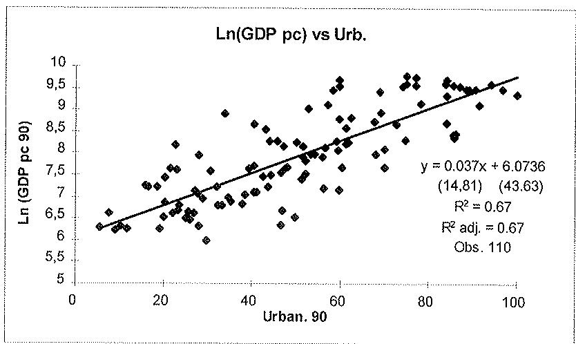
It is an obvious fact that the countries with the greatest gross domestic product per capita are also those with the greatest urbanization rate. Under the hypothesis that all other variables remain constant, (Ceteris Paribus hypothesis) this would indicate a greater productivity in the more urbanized countries, and therefore a greater efficiency level of those countries. As can be appreciated in the following figure, this relationship is exponential and very significant.
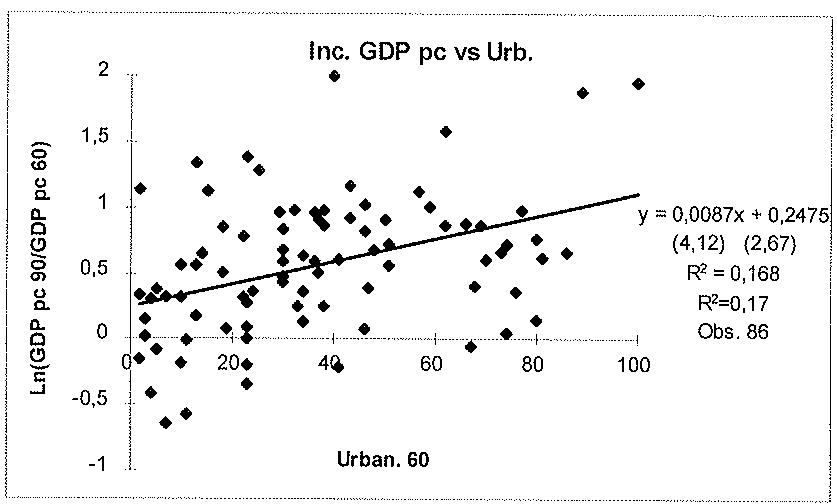
Concerning economic growth, we observe that the most urbanized countries in 1960 have experienced a higher growth rate during the 1960 - 1990 period. See figure below.
4 THE NEOCLASSICAL GROWTH MODEL AND EXOGENOUS URBANIZATION
Following the recent restatement of the ability of the neoclassical growth model to explain economic growth, due mainly to the contributions of Romer (1986) and Lucas (1988, 1993), in this section, I develop a simple neoclassical model in which the externalities linked to the exogenous urbanization rate are explicitly modelled.
I consider a simple economy in which a single product is produced with the following production function whose inputs are physical capital, and effective labour units.
\[Y _ {t} = F (K _ {t}, A _ {t} N _ {t})\]
Effective labour is the number of workers in the economy , that is assumed to be constant, multiplied by a measure of their human capital content reflected in . Let:
\[\frac {d A _ {t}}{d t} = A _ {t} g (u _ {t})\]
So that the technical change is labour-saving in the Harrod sense.
The production function is continuous, twice differentiable and with constant returns to scale and therefore first degree homogeneous. Given these, the production function can be expressed as:
\[y _ {t} = f (k _ {t}) \text {with} f ^ {\prime} (k) > 0 \text {and} f ^ {\prime \prime} (k) \leq 0.\]
Small letters represent the variable per unit of effective labour.
I also assume that there is no population growth or physical capital depreciation.
Production is devoted to consumption and capital accumulation (net investment):
\[Y _ {t} = C _ {t} + I _ {t}, \text { with } I _ {t} = \frac {d K _ {t}}{d t}\]
Eaton and Eckstein mention in their 1993 paper that large cities will have higher levels of human capital, also Rauch, 1991: "... my results reflect productivity benefits from geographic concentration of human capital caused by sharing of ideas".
Or in per-capita terms:
\[f (k _ {t}) = c _ {t} + \frac {d k _ {t}}{d t} + g (u _ {t}) k _ {t}.\tag{1}\]
The optimal control problem that the consumer must solve to obtain the global maximum is:
\[\left. \begin{array}{c} M a x \int_ {0} ^ {\infty} U (c _ {t}) e ^ {- \theta t} d t \\ f (k _ {t}) = c _ {t} + \dot {k} _ {t} + g (u _ {t}) k _ {t} \\ c _ {t} \geq 0 \\ k _ {t} \geq 0 \end{array} \right\}\]
Where is the discount factor.
The Hamiltonian function is defined by:
\[H _ {t} = U (c _ {t}) e ^ {- \theta t} + \mu_ {t} (f (k _ {t}) - c _ {t} - g (u _ {t}) k _ {t})\]
Or
\[H _ {t} = U (c _ {t}) e ^ {- \theta t} + \lambda_ {t} e ^ {- \theta t} (f (k _ {t}) - c _ {t} - g (u _ {t}) k _ {t})\]
With . The conditions for solving this problem are:
\[\begin{array}{r l} & {1. \frac {d v _ {t}}{d t} = - H _ {k} \Rightarrow \dot {\lambda} _ {t} e ^ {- \theta t} - \lambda_ {t} \theta e ^ {- \theta t} = - \lambda_ {t} e ^ {- \theta t} (f ^ {\prime} (k _ {t}) - g (u _ {t})) \dot {\lambda} _ {t} =} \\ & {\qquad \lambda_ {t} \theta - \lambda_ {t} f ^ {\prime} (k _ {t}) + \lambda_ {t} g (u) = - \lambda_ {t} (f ^ {\prime} (k _ {t}) - \theta - g (u))} \end{array}\]
\[2. H _ {c} = 0 \Rightarrow U ^ {\prime} (c _ {t}) = \lambda_ {t}\]
3. (transversality condition)
Solving this system:
\[\begin{array}{c} (U ^ {\prime} (c _ {t})) = - U ^ {\prime} (c _ {t}) [ (f ^ {\prime} (k _ {t}) - \theta - g (u)) ] \Rightarrow \\ \frac {U ^ {\prime \prime} (c _ {t}) c _ {t}}{U ^ {\prime} (c _ {t})} = \theta + g (u) - f ^ {\prime} (k _ {t}) \end{array}\tag{2}\]
The sole member of the family of paths satisfying both the initial conditions and the transversality condition is the optimal path.
To fully work out the predictions of the model we need specific production and utility functions, let these functions be:
\[U (c _ {t}) = \frac {c _ {t} ^ {1 - \gamma}}{1 - \gamma}\]
(constant risk adversion, )
\[F (K, L) = K _ {t} ^ {\alpha} L _ {t} ^ {(1 - \alpha)} \Rightarrow f (k) = k ^ {\alpha} \Rightarrow f ^ {\prime} (k _ {t}) = \alpha k ^ {(\alpha - 1)}\]
so that in place of equation (2) we have:
\[\frac {\dot {c} _ {t}}{c _ {t}} = - \frac {1}{\gamma} (\theta + g (u) - f ^ {\prime} (k _ {t}))\]
Or:
\[\alpha k ^ {(\alpha - 1)} = \gamma \frac {\dot {c} _ {t}}{c _ {t}} + \theta + g (u)\tag{3}\]
Using equation (1) we can solve the system to obtain:
\[\frac {c _ {t} + \frac {d k _ {t}}{d t} + g (u _ {t}) k _ {t}}{k _ {t}} = \frac {\gamma \frac {\dot {c} _ {t}}{c _ {t}} + \theta + g (u)}{\alpha} \Rightarrow \frac {c _ {t}}{k _ {t}} = - \frac {\dot {k} _ {t}}{k _ {t}} + \frac {\gamma \frac {\dot {c} _ {t}}{c _ {t}} + \theta + g (u) (1 - \alpha)}{\alpha}\]
As the right hand side of the previous equation is constant through the balance consumption path we can differentiate to obtain:
\[\frac {\dot {c}}{c} = \frac {\dot {k}}{k}\]
we can also differentiate equation (3) to obtain:
\[g (u) = \frac {\dot {K}}{K}\]
Hence, along the balanced path, the rate of growth is a function of the urbanization rate.
At the steady state , we can solve equations (2) and (3):
to obtain the constant balanced per capita value of the following variables; capital, consumption and savings:
\[k ^ {*} = \left(\frac {\theta + g (u)}{\alpha}\right) ^ {\frac {1}{1 - \alpha}}\]
\[c ^ {*} = \left(\frac {\theta + g (u)}{\alpha}\right) ^ {\frac {1}{1 - \alpha}} \left(\frac {\theta + g (u) (1 - \alpha)}{\alpha}\right)\]
\[s ^ {*} = g (u) \left(\frac {\theta + g (u)}{\alpha}\right) ^ {\frac {1}{1 - \alpha}}\]
According to this model, the rate of long term growth, for both the physical capital stock and the per capita production, is , so the economy with a greater urbanization rate, therefore with more cross fertilization, technological and knowledge externalities, will grow faster. So in a given economy if we vary the urbanization rate it will vary the growth rate.
In this model two economies with different urbanization rates will have a different long term balance growth rate.
5 ENDOGENOUS URBANIZATION
In this section I study the characteristics and behavior of an endogenous urbanization growth model. Martin and Ottaviano (1996) use also an endogenous growth model to conclude that with local spillovers the economic activity agglomerates and the rate of technological progress increases.
5.1 THE GENERAL MODEL
Let the production functions of a homogeneous product in the center (cities) and in the periphery be:
\[Y _ {c, t} = A _ {c, t} L _ {c, t} ^ {\alpha}\]
\[Y _ {p, t} = A _ {p, t} L _ {p, t} ^ {\alpha}\]
If we consider that the real wages are equal throughout the economy , we can use the first order conditions of profit maximization to obtain:
Therefore: .
Perfect mobility of labour demand and supply.
This result can also be obtained under the assumption of perfect competition.
\[\left(\frac {L _ {c , t}}{L _ {p , t}}\right) ^ {\alpha - 1} = \frac {A _ {p , t}}{A _ {c , t}}\tag{4}\]
The evolution of the technology in the center is a function of the urbanization rate according to the following differential equation:
\[\frac {d A _ {c , t}}{d t} = A _ {c, t} g \left(\frac {L _ {c}}{L _ {c} + L _ {p}}\right)\]
where g is a linear function of the urbanization rate with and positive negative or equal to cero, so that:
\[A _ {c, t} = A _ {c, 0} e ^ {g \left(\frac {L _ {c}}{L _ {c} + L _ {p}}\right) t}\]
From now on, in this work, we will consider that is equal to .
In accordance with the "catch-up" literature (de la Fuente, 1995), We assume that the evolution of the technological progress at the periphery is a function of the technological distance between center and periphery and has this function:
\[\frac {d A _ {p , t}}{d t} = A _ {p, t} b \log \left(\frac {A _ {c , t}}{A _ {p , t}}\right)\]
In the steady state, the growth rate of the technology, and therefore the economy's growth rate in equilibrium, are the same for the center and the periphery:
\[\frac {\frac {d A _ {c , t}}{d t}}{A _ {c , t}} - \frac {\frac {d A _ {p , t}}{d t}}{A _ {p , t}} = g (u) - b \log \left(\frac {A _ {c , t}}{A _ {p , t}}\right) = 0\]
Using equation(4) we can solve the system to obtain the urbanization rate in the steady state:
\[\left(\frac {u}{1 - u}\right) \equiv e ^ {\frac {x u}{h (1 - \alpha)}}\]
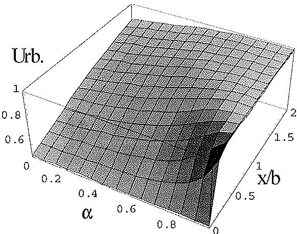
The urbanization rate is an implicit function of three variables, the speed of the "catch up" b, the technological progress deriving from the urbanization x, and the labour intensity of the production function . The following figure shows the evolution of the percentage of the population living in centers according to these parameters.
The figure shows an urbanization rate that is an increasing function of the labour intensity of the production function (0 < < 1) and of the rate of technological progress, or in other words, the urbanization rate is an increasing function of the positive external effects deriving from urbanization. A greater intensity of knowledge spillover implies a greater population percentage that would like to benefit from this positive externality. The rate of knowledge diffusion or technological "catch up" has a negative effect on the urbanization rate, it is a centripetal force. A faster technological diffusion from the center to the periphery, that is a shorter lag between the generation of a new technology in the center and the use of this technology in the periphery, implies lower urbanization and growth rates. The greater the diffusion rate, the lower the interest that people have in going to where the technology is generated, since in a short period of time, these people, living at the periphery, will be able to use the new technologies. In this case it is more interesting to make use of the lower intensity of labour that exists at the periphery.
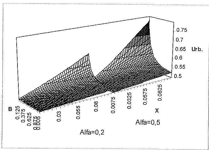
The derivates of the urbanization rate are the ones mentioned under the following general conditions: b > 0, x > 0 y 0 < .
5.2 EXTENSIONS OF THE ENDOGENOUS URBANIZATION MODEL
5.2.1 CENTRIPETAL AND CENTRIFUGAL FORCES
The first and maybe the most obvious extension of the model is the inclusion of centripetal-centrifugal forces that weaken or reinforce the urbanization in a territory producing a lower or a greater steady state urbanization rate. Let us suppose that the technology in the center has some congestion cost, , that decreases the technology growth rate. In this case the technology in the center behaves according to:
\[\frac {d A _ {c , t}}{d t} = A _ {c, t} \left[ g (u) - \tau \right]\]
At the periphery we have the same technology behavior:
\[\frac {d A _ {p , t}}{d t} = A _ {c, t} b \log \left(\frac {A _ {c , t}}{A _ {p , t}}\right)\]
In this model the fraction of people in the center over the people living in the periphery in the steady state is:
\[\left(\frac {u}{1 - u}\right) = e ^ {\frac {x u - \tau}{(1 - \alpha) b}}\]
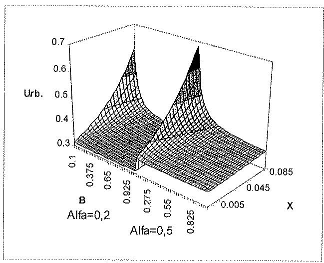
Consequently, the urbanization rate is lower when the transaction costs are greater . The urbanization rate has a negative relationship with the centrifugal forces and a positive one with the centripetal forces. Figure (2) is similar to figure (1). We can observe that the inclusion of congestion costs causes a non-linear decrease in the steady state urbanization rate.
... a decrease of transaction costs, through for example trade integration, will increase the growth rate because it leads a higher industrial concentration of firms where the R&D is located." Martin and Ottaviano (1996).
Figure 2:
5.2.2 TECHNOLOGICAL DIFFUSION AND URBANIZATION
We can consider that the technological diffusion parameter b, depends on the urbanization rate. The spread of technology from the center to the periphery is faster when there are proportionally less people living at the periphery. If we consider that the technological diffusion is a linearly increasing function of the urbanization rate the problem becomes easier. We would have the following behavioral rule for the urbanization rate:
\[\frac {u}{1 - u} = e ^ {\frac {\frac {x}{b}}{1 - \alpha}}\tag{5}\]
In this case the population living in the center is an increasing function of and of . This equation is plotted in figure (3), where we can notice how the urbanization rates vary when the parameters change.
Under the general conditions mentioned above, the urbanization rate depends on the parameters in the same way that we found previously. The urbanization is a continuous function increasing on x and and decreasing on b.
5.2.3 URBANIZATION AND TIME
In this sort of model, a variation of the urbanization rate in the steady state over time is only produced either through the endogeneization of the parameters, for instance the parameters can be a function of the technological level, or through exogenous variations in the parameters of the model.
If the congestion cost decreases with the technological level, the urbanization rate will increase with time. If the rate of technological diffusion increases with the technological level, the urbanization will decrease with time.
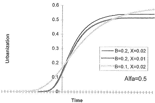
Outside the steady state, that is with different growth rates for the center and the periphery, we can easily obtain the evolution of the urbanization rate over time in a particular case of the model with . In this case, the technology in the center and in the periphery is:
\[A _ {c, t} = A _ {c, 0} e ^ {x t}\]
\[A _ {p, t} = e ^ {\left(K e ^ {- b t}\right) + \log A _ {c, 0} - \frac {x}{b} + x t}\]
With the condition of equal real wages across the economy, equation (4), we can obtain an implicit function of the evolution of the urbanization rate:
\[\left(\frac {u}{1 - u}\right) ^ {1 - \alpha} = e ^ {\frac {x}{b} - k e ^ {- b t}}\tag{6}\]
Note that when , then and we have the previous section case, the steady state of the urbanization rate.
We can clear in equation (6) to obtain:
\[t = \frac {- L n \left(\frac {x}{b} - (1 - \alpha) (L n (u) - L n (1 - u))\right)}{b}\]
The following figure shows the evolution of the urbanization rate using the previous equation for different values of the parameters.
Figure 4:
6 EMPIRICAL ANALYSIS
A lot of variables have been introduced in theoretical neoclassical endogenous growth models and found to be significant in a number of empirical specifications. The level of human capital plays a significant role in a great number of these models. Human capital both, promotes innovations and makes it easier to absorb the new technologies discovered elsewhere. Therefore a country with a higher level of human capital tends to grow faster.
In the theoretical model presented, we also find that a greater urbanization rate is positively correlated with the growth rate. We know that the concentration of the population facilitates the transmission and cross fertilization of ideas, thus increasing the underlying technological progress. Our empirical model must include this fact, therefore the growth of the real GDP per capita should be an increasing function of the urbanization rate. We also must include the well documented fact of convergence across economies predicted by the Neoclassical Growth Model. And finally we must include the human capital variable to be sure that the urbanization rate variable is not significant because it is gathering the effect of human capital stock on growth .
The data used in this section are from Summers and Heston, Penn World Table (mark 5.6) and from the World Bank data base. From the World Bank we use the value of the real per capita GDP (chain index) expressed in international prices, base 1985 and the real investment share of GDP. The human capital variable is defined as the number of students enrolled in secondary school as a percentage of the total population of the corresponding age group. Although in our data set we have not any case, note that it would be possible to have an index for this variable greater than 100. Finally our variable of agglomeration will be the total urban population as a percentage of the total population of the country.
Table (1) presents the results of the estimation, for the following equation of GDP growth across countries:
I also tried the rate of industry on GDP, the estimation does not vary significantly.
Note that different countries have a different definitions of urbanization according to what they consider urban population for their country.
\[L o g \left(\frac {G r o w t h G D P}{T}\right) = \alpha - \frac {1 - e ^ {- \beta T}}{T} L o g (G D P p c 6 0) + \gamma * S E C 6 0 + \delta * U R B 6 0 + \xi\tag{7}\]
| GDP growth per capita between 1960 and 1990 | |||
| Constant | 0.056 | 0.053 | 0.096 |
| (3.38) | (2.65) | (4.54) | |
| GDP per capita in 1960 | 0.007 | 0.008 | 0.017 |
| (2.38) | (1.94) | (3.09) | |
| Secondary school enrolment 1960 | 0.051 | 0.042 | |
| (4.64) | (3.73) | ||
| Urbanization rate 1960 | 0.047 | 0.039 | |
| (3.73) | (2.96) | ||
| $R^2$ adj | 0.19 | 0.21 | 0.31 |
| Obs. | 82 | 82 | 82 |
| T statistics are in parentheses $^{13}$ . | |||
Following Mankiw, Romer and Weil (1992) and including the external effect due to urbanization we obtain (see appendix 1):
\[L o g (G D P p c) = C t e - \beta_ {1} L o g (n + f + \delta) + \beta_ {2} L o g (s _ {k}) + \beta_ {3} L o g (s _ {h}) + \beta_ {4} U r b + \xi\tag{8}\]
Table (2) shows the annual influence on the GDP per capita steady state of each variable, according to the previous model:
The t-statistics are calculated with standard errors robust to heterocedasticity, based on White (1980) heteroskedasticity-consistent covariance matrix.
According to the results of the estimations of equations (7) and (8) we find evidence of positive external effects deriving from the agglomeration of economic activity. The countries with a higher urbanization rate in 1960 have grown more in the 1960-1990 period, and during these years the countries more urbanized have had greater steady state growth rates.
| GDP per capita 1990 | |||
| Constant | -0.32 | 3.71 | 3.38 |
| (0.22) | (2.92) | (3.12) | |
| Ln (n+ f+δ) | -3.61 | -2.04 | -1.64 |
| (7.39) | (4.62) | (4.29) | |
| LN (I/GDP) | 0.69 | 0.23 | 0.15 |
| (7.03) | (2.33) | (1.73) | |
| Ln (sec. school enrolment) | 0.72 | 0.37 | |
| (8.35) | (3.86) | ||
| Urb. Rate | 1.94 | ||
| (6.03) | |||
| R2adj | 0.61 | 0.76 | 0.83 |
| Obs. | 104 | 104 | 104 |
| F-test | 10.61 | 108.76 | 128.58 |
| T statistics are in parentheses14. | |||
| f + δ = 0.05 following Mankiw, Romer and Weil (1992) | |||
7 CONCLUSIONS
In this paper I have provided a new approximation to the study of economic agglomerations. I propose a variety of neoclassical growth models to study agglomeration and the effects of the external economies deriving from it. In these models the technological externalities (knowledge spillovers, cross fertilization of ideas ...) that urbanization generates, are the source of growth of the economy. This prediction is in accordance with the empirical correlation between growth and urbanization rates.
In a second stage, an endogenous growth model, with technological diffusion from the center to the periphery, is worked out. This model shows a negative effect of the speed of technological diffusion on urbanization rate and consequently on growth. A dynamic environment of production of externalities and greater intensity of labour in the production function creates higher urbanization rates.
The t-statistics are calculated with standard errors robust to heterocedasticity, based on White (1980) heteroskedasticity-consistent covariance matrix.
The empirical results document a positive effect of urbanization on both GDP growth and GDP per capita steady state. These findings support the theories of external effects due to agglomeration. Cities are centers in which the generation of externalities is enhanced and fostered by the cross fertilization and transmission of ideas.
Economic activity tends to agglomerate because it produces a higher growth rates through technological external effects generated in the agglomerations. The steady state agglomeration rate will depend on the intensity of the external effects and of the centripetal, centrifugal forces, and it can vary over time only if the economy is not in the steady state or if the parameters also vary. Policies that foster higher steady state urbanization rates will provoke higher long run growth rates.
References
- [1] Ades, A. F. and Glaeser, E. L. (1994): "Evidence on Growth, Increasing Returns and the Extent of the Market", Working Paper No. 4714. National Bureau of Economic Research.
- [2] Azariadis, C. (1993): Intertemporal Macroeconomics. Blackwell.
- [3] Bairoch, P. (1988): Cities and Economic Development. Chicago, Univ. Chicago Press.
- [4] Ciccone, A. and Hall, R. E. (1993): "Productivity and the Density of Economic Activity" Working Paper No. 4313. National Bureau of Economic Research.
- [5] de la Fuente, A (1995): "Catch-up, growth and convergence in the OCDE" Working Paper No. 1274. Center for Economic Policy Research.
- [6] Eaton, J. and Eckstein Z. (1993): "Cities and Growth: Theory and Evidence from France and Japan" CEPR conference, Trade and Growth organized by: CEPR, Institut d'Análisi Económica and Universitat Pompeu Fabra.
- [7] Ellison, G. (1993): "Learning, Local Interaction, and Coordination" Econometrica Vol. 16 No. 5.
- [8] Ellison, G. and Glaeser E. L. (1994): "Geographic Concentration in .US. Manufacturing Industries: A Dartboard Approach" Working Paper No. 4840. National Bureau of Economic Research.
- [9] Glaeser, E.L.(1994):"Cities, Information and Economic Growth", Discussion Paper No. 1681, Harvard Institute of Economic Research, Cambridge.
- [10] Glaeser, E.L. and Maré, D.C. (1994): "Cities and Skills" Working Paper No. 4728. National Bureau of Economic Research.
- [11] Glaeser, E. L.; Scheinkman, J. A. and Shleifer, A. (1995): "Economic Growth in a Cross-Section of Cities", Journal of Monetary Economics, Vol.36, pp.117-143.
- [12] Grossman, G.M. and Helpman, E. (1991): Innovation and Growth in the global Economy. Cambridge, Massachusetts. The MIT press.
- [13] Hall, R. (1989): "Temporal Agglomeration". Working Paper No. 3143. National Bureau of Economic Research.
- [14] Jacobs, J. (1969): The Economy of Cities. New York: Vintage.
- [15] Krugman, P. (1991): "Increasing Returns and Economic Geography" Journal of Political Economy. Vol. 99, pp. 483-499.
- [16] Krugman, P. (1991): Geography and Trade. Cambridge: MIT Press.
- [17] Krugman, P. and Livas, R. (1992): "Trade Policy and the Third World Metropolis." Working Paper No. 4238. National Bureau of Economic Research.
- [18] Lucas, R. J. (1988): "On the Mechanics of Economic Development", Journal of Monetary Economics, No. 22, pp. 3-42.
- [19] Lucas, R. J. (1993): "Making a Miracle" Econometrica No. 61.
- [20] Martin, P. and Ottaviano, G. (1996): "Growing Locations: Industry Location in a Model of Endogenous Growth", CEPR Discussion Paper, No. 1523.
- [21] Marshall, A. (1890): Principles of Economics. London. Macmillan.
- [22] Rauch, J. E. (1991): "Productivity Gains from Geographic Concentration of Human Capital: Evidence from the Cities" Working Paper No. 3905. National Bureau of Economic Research.
- [23] Romer, P. (1986): "Increasing Returns and Long-Run Growth", Journal of Political Economy, Vol. 94, No. 5.
- [24] Romer, P. (1990): "Endogenous technological Change", Journal of Political Economy, Vol. 98, No. 5.
- [25] Solow, R. M. (1956):” A Contribution to the Theory of Economic Growth.” The Quartely Journal of Economics, No. 70, pp.65-94.
APPENDIX I
ANALYTICAL SOLUTION OF THE ENDOGENOUS URBANIZATION RATE MODEL.
First I have to solve the differential equation for .
Consider the following equation:
\[\frac {d A _ {p , t}}{d t} = A _ {p, t} b \log \left(\frac {A _ {c , t}}{A _ {p , t}}\right)\]
With we have:
\[\frac {d A _ {p , t}}{d t} = A _ {p, t} b \log \left(A _ {c, 0} e ^ {\left(\frac {L _ {c}}{L _ {c} + L _ {p}}\right) x t}\right) - A _ {p, t} b \log A _ {p, t}\]
We can make the following variable change and obtain:
\[\frac {d Z}{d t} = b \log A _ {c, 0} + b \left(\frac {L _ {c}}{L _ {c} + L _ {p}}\right) x t - b Z\]
Now we can solve this differential equation.
Homogeneous equation solution:
\[\frac {d Z}{d t} = - b Z \Rightarrow Z = k e ^ {- b t}\]
Particular solution of the general equation:
\[\frac {d Z}{d t} = \frac {d k (t)}{d t} e ^ {- b t} - k (t) b e ^ {- b t} = b \log A _ {c, 0} + b \left(\frac {L _ {c}}{L _ {c} + L _ {p}}\right) x t - b k (t) e ^ {- b t}\]
\[\frac {d k (t)}{d t} = e ^ {b t} \left(b \log A _ {c, 0} + b \left(\frac {L _ {c}}{L _ {c} + L _ {p}}\right) x t\right)\]
\[k (t) = e ^ {b t} \left(\log A _ {c, 0} - \frac {\left(\frac {L _ {c}}{L _ {c} + L _ {p}}\right) x}{b} + \left(\frac {L _ {c}}{L _ {c} + L _ {p}}\right) x t\right)\]
General solution of the equation:
\[Z = k e ^ {- b t} + \left(\log A _ {c, 0} - \frac {\left(\frac {L _ {c}}{L _ {c} + L _ {p}}\right) x}{b} + \left(\frac {L _ {c}}{L _ {c} + L _ {p}}\right) x t\right)\]
We can undo the variable change to obtain :
\[A _ {p, t} = e ^ {Z} = e ^ {\left(k e ^ {- b t} + \log A _ {c, 0} - \frac {\left(\frac {L _ {c}}{L _ {c} + L _ {p}}\right) ^ {x}}{b} + \left(\frac {L _ {c}}{L _ {c} + L _ {p}}\right) x t\right)}\]
We can now substitute this equation in the real wage equation and in the growth rate equation:
\[\left(\frac {L _ {c}}{L _ {p}}\right) ^ {1 - \alpha} = \frac {A _ {c , 0} e ^ {\left(\frac {L _ {c}}{L _ {c} + L _ {p}}\right) x t}}{e ^ {(k e ^ {- b t})} e ^ {\log A _ {c , 0}} e ^ {- \frac {\left(\frac {L _ {c}}{L _ {c} + L _ {p}}\right) x}{b}} e ^ {\left(\frac {L _ {c}}{L _ {c} + L _ {p}}\right) x t}} = e ^ {- k e ^ {- b t} + \frac {\left(\frac {L _ {c}}{L _ {c} + L _ {p}}\right) x}{b}}\]
\[\left(\frac {L _ {c}}{L _ {c} + L _ {p}}\right) x t + k e ^ {- b t} - \frac {\left(\frac {L _ {c}}{L _ {c} + L _ {p}}\right) x}{b} = 0\]
Therefore:
\[\left(\frac {L _ {\mathrm{c}}}{L _ {p}}\right) ^ {\alpha - 1} = e ^ {\frac {\left(\frac {L _ {c}}{L _ {\mathrm{c}} + L _ {p}}\right) x t}{b}}\]
When :
it readily obtained.
STEADY STATE INCOME PER CAPITA EQUATION.
Following Mankiw, Romer and Weil's (1992) work, let the production function be:
\[Y _ {t} = K _ {t} ^ {\alpha} H _ {t} ^ {\beta} (E _ {t} A _ {t} L _ {t}) ^ {1 - \alpha - \beta}\]
Where is the stock of externalities due to agglomeration produced each period and it is assumed to be a function of u :
\[E _ {t} = E _ {0} e ^ {g (u)}\]
L and A grow at rates n and f according to the following functions:
\[L _ {t} = L _ {0} e ^ {n t}\]
\[A _ {t} = A _ {0} e ^ {f t}\]
The production function per effective unit of labor, defined as is:
\[y = k ^ {\alpha} h ^ {\beta} E _ {t} ^ {(1 - \alpha - \beta)}\]
Let us consider that a constant fraction of output is invested in physical capital , and in human capital . With a depreciation rate of , the evolution of this economy is determined by the following two equations:
\[\begin{array}{l} \dot {k} = s _ {k} y - (n + \delta + f) k \\ \dot {h} = s _ {h} y - (n + \delta + f) h \end{array}\]
In the steady state . Therefore:
\[\left\{ \begin{array}{l l} k = (s _ {k} h ^ {\beta} E _ {t} ^ {1 - \alpha - \beta} / (n + \delta + f)) ^ {1 / (1 - \alpha)} \\ h = (s _ {h} k ^ {\alpha} E _ {t} ^ {1 - \alpha - \beta} / (n + \delta + f)) ^ {1 / (1 - \beta)} \end{array} \right.\]
Substituting within these equations:
\[k = \left(\frac {s _ {k} \left(\frac {s _ {h} k ^ {\alpha} E _ {t} ^ {1 - \alpha - \beta}}{(n + \delta + f)}\right) ^ {\beta / (1 - \beta)} E _ {t} ^ {1 - \alpha - \beta}}{(n + \delta + f)}\right) ^ {1 / (1 - \alpha)} = \left(\frac {s _ {k} ^ {(1 - \beta)} s _ {h} ^ {\beta} k ^ {\beta \alpha} E _ {t} ^ {1 - \alpha - \beta}}{n + \delta + f}\right) ^ {1 / (1 - \beta) (1 - \alpha)} \Rightarrow\]
\[k ^ {*} = \left(\frac {s _ {k} ^ {(1 - \beta)} s _ {h} ^ {\beta} E _ {t} ^ {1 - \alpha - \beta}}{n + \delta + f}\right) ^ {1 / (1 - \beta - \alpha)} \mathrm{and} h ^ {*} = \left(\frac {s _ {k} ^ {\alpha} s _ {h} ^ {(1 - \alpha)} E _ {t} ^ {1 - \alpha - \beta}}{n + \delta + f}\right) ^ {1 / (1 - \beta - \alpha)}\]
Substituting into the production function the steady states of k, and h and taking logs:
\[L o g (Y / L) = L o g (A _ {0} * E _ {0}) + g t - \frac {\alpha + \beta}{1 - \alpha - \beta} L o g (n + f + \delta) +\]
\[+ \frac {\alpha}{1 - \alpha - \beta} L o g (s _ {k}) + \frac {\beta}{1 - \alpha - \beta} L o g (s _ {h}) + (1 - \alpha - \beta) g (u)\]
APPENDIX III
COUNTRIES IN REGRESSIONS
Name: 1 (observation in the 30 years growth model); 1 (observation in the 30 years GDP per capita model)
Algeria :1;1. Argentina :1;1. Australia :1;1. Austria :1;1. Bangladesh :1;1. Belgium :1;1. Benin :1;1. Bolivia :1;1. Brazil :1;1. Bulgaria :0;1. Burkina Faso :0;1. Burundi :1;1. Cameroon :1;1. Canada :1;1. Cape Verde Is. :0;1. Central Afr. :1;1. Chad :0;1. Chile :1;1. China :1;1. Colombia :1;1. Comoros :0;1. Congo :1;1. Costa Rica :1;1. Cyprus :0;1. Denmark :1;1. Dominican Rep. :1;1. Ecuador :1;1. Egypt :1;1. El Salvador :1;1. Fiji :0;1. Finland :1;1. France :1;1. Gabon :0;1. Gambia :0;1. Ghana :1;1. Greece :1;1. Guatemala :1;1. Guinea :1;1. Guinea-Biss :0;1. Guyana :0;1. Honduras :1;1. Hong Kong :1;1. Hungary :0;1. Iceland :0;1. India :1;1. Indonesia :1;1. Iran :1;1. Ireland :1;1. Israel :1;1. Italy :1;1. Ivory Coast :1;1. Jamaica :1;1. Japan :1;1. Jordan :1;1. Kenya :1;1. Laos :0;1. Lesotho :1;1. Luxembourg :0;1. Madagascar :1;1. Malawi :1;1. Malaysia :1;1. Mali :1;1. Mauritania :0;1. Mauritius :0;1. Mexico :1;1. Mongolia :0;1. Morocco :1;1. Mozambique :1;1. Namibia :0;1. Netherlands :1;1. New Zealand :1;1. Nicaragua :1;1. Nigeria :1;1. Norway :1;1. Pakistan :1;1. Panama :1;1. Papua N. Guinea :1;1. Paraguay :1;1. Peru :1;1. Philippines :1;1. Poland :0;1. Portugal :0;1. Rwanda :1;1. Senegal :1;1. Sierra Leone :0;1. Singapore :1;1. South Africa :1;1. Spain :1;1. Sri Lanka :1;1. Sudan :0;1. Sweden :1;1. Switzerland :1;0. Syria :1;1.Thailand :1;1. Togo :1;1. Trinidad And Tobago :1;1. Tunisia :1;1. Turkey :1;1.U.K.: 1:2 U.S.A.: 2:2 Uganda :2:2 Uruguay :2:2 Venezuela :2:2 Zambia :2:2 Zimbabwe :2:2
COLECCION RESUMENES
96-02: “Evidencia empírica de sustituibilidad entre los componentes sectoriales del ahorro nacional en algunos países de la Unión Europea”, Isabel Argimón.
96-01: "El mercado de depósitos español (1985-1994): Bancos versus Cajas de Ahorro", Juan Coello.
95-01: “Geografía económica y política territorial”, CEP, FEDEA (Coordinador), IKEI e IVIE.
TEXTOS EXPRESS
96-02: “La Unión Económica y Monetaria en Europa”, encuesta coordinada por: Miguel Sebastián y Simón Sosvilla.
96-01: "La Seguridad Social del siglo XXI y la reforma de las pensiones de 1996", José A. Herce.
DOCUMENTOS DE TRABAJO
96-28: “Urbanization and growth”, Juan J. de Lucio.
96-27: "Efectos macroeconómicos del mercado único europeo: Un análisis basado en el modelo HERMIN", Simón Sosvilla-Rivero y José Antonio Herce.
96-26: “Capacity and access pricing strategies: An argument for the liberalization of telecommunication infrastructure”, A. Urbano, G. Olcina y Y. Tauman.
96-25: “La reforma de las pensiones en España: Aspectos analíticos y aplicados”, José A. Herce.
96-24: “Transitional Effects of a Pension System Change in Spain”, José M. Bailén y Joan Gil.
96-23: “Convergencia real en la Unión Europea: Un análisis de series temporales”, Vicente Esteve y Vicente J. Pallardó.
96-22: “Monetary union and european unemployment”, José Viñals y Juan F. Jimeno.
96-21: “El equilibrio financiero de un sistema de reparto de pensiones de jubilación: Una aplicación al caso español”, Juan F. Jimeno y Omar Licandro.
96-20: “The effects of migration on the relative demand of skilled versus unskilled labour: Evidence from Spain”, Juan J. Dolado, Juan F. Jimeno y Rosa Duce.
96-19: “The causes of Spanish unemployment: A structural VAR approach”, Juan J. Dolado y Juan F. Jimeno.
96-18: “La Unión Económica y Monetaria en Europa: Una encuesta entre expertos académicos y de mercados”, Miguel Sebastián y Simón Sosvilla.
96-17: “Externalities and growth in the Spanish industries”, Berta Moreno.
96-16: "Replacement echoes in the vintage capital growth model", Raouf Boucekkine, Marc Germain and Omar Licandro.
96-15: "La industria en las Comunidades Autónomas: 1978-1992", José A. Herce, Juan J. de Lucio y Ana Goicolea.
96-14: "Externalities and industrial growth: Spain 1978-1992", Juan J. de Lucio, José A. Herce y Ana Goicolea.
96-13: “Bases para profesionalizar la sanidad pública”, Benito Arruñada.
96-12: "Capacity utilization and market power", J-Fr. Fagnart, Omar Licandro y H. R. Sneessens.
96-11: "Idiosyncratic uncertainty, capacity utilization and the business cycle", Frank Portier, Omar Licandro, y Jean François Fagnart.
96-10: “La financiación privada de los servicios sanitarios”, C. Murillo, S. Calonge e Y. González.
96-09: "Los efectos visibles de la reforma laboral de 1994", Juan F. Jimeno.
96-08: “Diseño y evaluación de estrategias de desregulación en el sector sanitario público en España”, Juan Manuel Cabasés Hita y José Martín Martín.
96-07: “Efectos de políticas macroeconómicas en una unión monetaria con distintos grados de rigidez salarial”, Carlos de Miguel Palacios y Simón Sosvilla-Rivero.
Este texto se ha extraído automáticamente del documento original. Para citarlo o leerlo con su maquetación, descargue el PDF.
Descargar en PDF