Statistical modeling of fishing activities in the North Atlantic by Carmen Fernández* Eduardo Ley** Mark F. J. Steel* DOCUMENTO DE TRABAJO 97-25
December, 1997
* CentER and Dept. of Econometrics, Tilburg University, The Netherlands.
** FEDEA
* CentER and Dept. of Econometrics, Tilburg University, The Netherlands.
This paper is available through Internet: http://www.fedea.es/hojas/publicaciones.html#Documentos de Trabajo
Statistical Modeling of Fishing Activities in the North Atlantic
Carmen Fernández , Eduardo Ley , and Mark F.J. Steel
CentER and Dept. of Econometrics, Tilburg University, The Netherlands, FEDEA, Madrid, Spain
Abstract. This paper deals with the issue of modeling daily catches of fishing boats in the Grand Bank fishing grounds. We have data on catches per species for a number of vessels collected by the European Union in the context of the North Atlantic Fisheries Organization. Many variables can be thought to influence the amount caught: a number of ship characteristics—such as the size of the ship, the fishing technique used, the mesh size of the nets, etc.—, are obvious candidates, but one can also consider the season or the actual location of the catch. In all, our database leads to 23 possible regressors, resulting in a set of possible linear regression models. Prediction of future catches and posterior inference will be based on Bayesian model averaging, using a Markov Chain Monte Carlo Model Composition (MC ) approach. Particular attention is paid to the elicitation of the prior and the prediction of catch for single and aggregated observations.
Keywords. Bayesian model averaging; Grand Bank fisheries; Predictive inference; Prior elicitation
"Fishing conflicts ara among the most visible of a new set of international security and diplomatic concerns caused by environmental degradation and resource depletion." [J. Friedland: "Catch of the Day: Fish Stories these Days are Tales of Depletion and Growing Rivalry," The Wall Street Journal, front page article, 25/11/97]
1. INTRODUCTION
The mismanagement of the world fisheries is one of the most important global environmental problems that we face today. In the early 90's, according to the
We wish to thank Fernando Tusell for useful comments and for kindly making the data available to us. We also acknowledge the cooperation of Alain Laurec of the European Commission DG-XIV-C in allowing us to use this data set. The first author was supported by a Training and Mobility of Researchers grant (\# ERBFMBICT 961021) awarded by the European Commission. This work was started when the second author was a Fellow at the Energy and Natural Resources Division of Resources for the Future, Washington D.C. The third author benefitted from a travel grant awarded by the Netherlands Organization for Scientific Research (NWO).
United Nations Food and Agriculture Organization (FAO), around 70% of the world's conventional species of fish were “fully exploited, overexploited, depleted, or in the process of rebuilding as a result of depletion” (FAO, 1995). Nine of the world's 17 major fisheries are in serious decline, and four others are classified as ‘commercially depleted’ by the FAO (Tibbets, 1994). By far, the largest single pressure on commercial fisheries is overexploitation, which occurs mostly due to the free open access to fishery resources. This lack of property rights then results in a tragedy of the commons (Hardin, 1968).
The North Atlantic Fisheries Organization (NAFO) is one of several international organizations that tries to alleviate overexploitation through voluntary cooperation. The NAFO was established in 1978 to contribute to the optimal exploitation and rational use of fisheries resources in the Grand Bank outside Canada's exclusive economic zone. Countries which are members of the NAFO (Bulgaria, Canada, Cuba, European Union -EU-, Federation of Russian States, Iceland, Japan, Letonia, Lithuania, Norway, Poland and Romania) assign quotas among themselves and grant inspection rights to each other. At present, there are three inspection ships —two Canadian and one belonging to the EU—that board vessels of member states and register the information in their logbooks. In addition, signatory countries' ships report (through the so-called "hails") their entry and exit of the different zones of the fishing grounds. Finally, there are two daily flights over the Grand Bank and the Flemish Cap made by inspection airplanes with the purpose of locating and identifying all ships fishing in the area (also including vessels from non-signatory countries).
However, boarding ships on high seas to verify catch is expensive and disrupts their operations. Furthermore, ships from non-signatory countries can not be inspected. It then becomes important to construct models that allow for catch prediction and monitoring conditional on the information from aerial sightings and hails, ship characteristics and other variables (such as month of the year). Improvement of the monitoring activities is crucial for the effectiveness of cooperative organizations such as NAFO. In addition, our model allows us to study how ship characteristics influence catch —correcting for other factors. The latter might provide useful information for regulatory measures and guidelines related to issues like net size, optimal size of the fleet, etc. An excellent introduction to the use of quantitative methods in fisheries research is given by Hilborn and Walters (1992).
This paper proposes a statistical model for daily catch per species of fish based on linear regression combined with a certain probability of zero catch. We work within a Bayesian framework and formally treat the uncertainty concerning the choice of regressors through model averaging, using posterior model probabilities as weights. In view of the large number of potential models, a Monte Carlo Markov chain is generated over the model space, following the MC methodology of Madigan and York (1995). Particular attention is paid to the choice of the prior, since we wish to combine a relative lack of prior information with feasible numerical calculations. Finally, efficient coding is seen to result in a software that can easily deal with problems of practically relevant dimensions.
Section 2 describes the data collected by the EU, while Section 3 introduces the statistical model, as well as model averaging. Posterior and predictive inference is discussed in Section 4, along with some details of the prior elicitation and the numerical implementation. The empirical results are presented in Section 5 and a final section concludes.
2. THE DATA
The original data were gathered by the inspection vessels of the EU operating on the Grand Bank fisheries. These vessels board the fishing boats and record basic characteristics of the ship and the fishing equipment, as well as the quantities caught of different species and where and when this catch was effectuated. They use the ship's logs to collect all the information accumulated since the last time the ship was boarded. All data correspond to 1993 and the first half of 1994, leading to 6806 observations corresponding to a particular ship at a given day. More information about the data and the way they are collected can be found in Ferreira and Tusell (1996). Figure 1 shows a map of the area in question. All available information relates to zones 3L, 3M, 3N and 3O.
In the recorded data, there are separate entries for ship type (6 categories), whether the ship was fishing alone or in a pair (2 categories), and the fishing technique (5 categories). Since the recorded data seem to be less than reliable in the exact categories of ship type (it is, e.g., not always correctly indicated whether a stern trawler has a freezer or not, and the same ships seem to change categories often), and there are some logical redundancies in these data (e.g., a pair trawl can only be used by ships fishing in a pair), we combine these three categorical variables into one single variable, with four levels, corresponding to the fishing technique used.
The dependent variable is the live weight of fish caught. Table 1 summarizes the regressors that we can possibly use. These include four categorical variables: the country where the vessel is registered, denoted by nationality (3 levels), fishing technique (4 levels), zone (4 levels) and month of the year (12 levels). Each of these variables is handled through dummies taking the values zero or one (with the possible exception of zone, as shall be described below). As the model will include an intercept, we retain one reference level for each of them. In addition, we have four continuous variables, namely net size measured in mm., length of vessel measured in m., gross registered tonnage (GRT) and engine kW. Table 1 indicates the empirical distribution of each of the categorical variables, and the means and standard deviations of each continuous variable, calculated over the sample of 6806 ship-days.
Table 2 lists the five most important species caught on the Grand Bank and has one category for all the other species (“rest”). Every time we observe a ship, we observe its daily catches for all six species. A look at the data tells us that a ship’s catch on any given day often does not include all six species. More in particular, the 6806 observed ship-days give us observations of catch per species, and 24,738 of these are zeros. This important aspect of the data should not be overlooked, and, hence, we shall model these zero catches explicitly. This feature of the data seems to have been ignored by Ferreira and Tusell (1996), who analyse the same data set. Table 2 also lists the percentage of zero observations per species and the fraction of the total live weight that each species constitutes. In dealing with this data set, a few other issues arise:

Table 1. Data Used
| Regressor | Description | % Observations | |
| 1 | Danish vessel | 0.4 | |
| 2 | Spanish vessel | 81.5 | |
| ref. | Portuguese vessel | 18.1 | |
| 3 | drift gillnet | 3.6 | |
| 4 | anchored gillnet | 1.4 | |
| 5 | otter trawl | 79.6 | |
| ref. | otter trawl pair | 15.4 | |
| 6 | zone 3L | 34.6 | |
| 7 | zone 3M | 25.7 | |
| 8 | zone 3N | 35.0 | |
| ref. | zone 3O | 4.7 | |
| 9 | January | 4.9 | |
| 10 | February | 10.7 | |
| 11 | March | 15.0 | |
| 12 | April | 12.1 | |
| 13 | May | 14.0 | |
| 14 | June | 9.5 | |
| 15 | July | 7.0 | |
| 16 | August | 7.7 | |
| 17 | September | 8.0 | |
| 18 | October | 7.0 | |
| 19 | November | 3.5 | |
| ref. | December | 0.6 | |
| Mean | Std | ||
| 20 | net size mm. | 125.99 | 7.02 |
| 21 | length vessel m. | 51.57 | 13.41 |
| 22 | GRT | 749.93 | 449.41 |
| 23 | engine kW | 1174.97 | 505.19 |
Table 2. Fish Species
| Sp. | Description | % zeros | % of catch |
| 1 | Atlantic cod (Gadus morhua) | 88.33 | 9.80 |
| 2 | Halibut (Hippoglossus reinhardtius)m | 18.50 | 62.40 |
| 3 | Redfish (Sebastes spp.) | 85.73 | 11.73 |
| 4 | Grenadier (Macrurus rupestris) | 43.20 | 3.80 |
| 5 | Skate (Raja spp.) | 55.44 | 8.97 |
| 6 | rest | 72.27 | 3.30 |
(i) Sometimes a ship is on the fishing grounds but is unable to do any fishing, due, e.g., to bad weather conditions. This is reflected in the data through a variable called: “# of fishing days”. If this variable takes a value, say K, bigger than one, it means that the previous K-1 days the ship was on the fishing grounds but could not fish. Thus, catch should be recorded as zero for all species during those K-1 days, whereas the amount registered in the logbook should be assigned to the day.
(ii) Another issue relates to the zone where the fish is caught. If a ship is in, e.g., 2 different zones during the same day, the logbook registers 2 entries on that day, each of them reflecting the amount of fish caught in that particular zone. Since we want to model the catch per ship per day, we shall sum (for each of the 6 species) the amount caught over all the zones visited. Then, in the explanatory variables, instead of imputing 1 for one of the zones, we assign the value to each of the zones visited. Although this is not fully precise, multiple zones in the same day occurs only very rarely in our dataset (1.2% of the observations).
Regarding the six different species mentioned in Table 2, there are different models that we could think of:
(i) We could model the total catch per ship-day, without separating per species. This would mean that for each ship, we sum the catch over all six species (leading to 6,806 observations in all). In the data, the total amount of catch is now always positive except when (\# of fishing days) > 1, which occurs in 8.2% of the observations. The fact that the data on the total amount of catch seems to be more reliable that its decomposition by species, is an advantage of such a modeling strategy. Nevertheless, for policy purposes, a model that can predict for each of the species seems more useful.
(ii) We could model catch per ship-day per species, by considering a single regression model and introducing a separate individual effect for each of the species, as in Ferreira and Tusell (1996). We remark that the total amount of observations is now since zero catches should not be neglected. The drawback of this model is that it seems somewhat unreasonable to assume that the explanatory variables affect all the species in the same way, and the species are only distinguished by a difference in the intercept. In the sequel, we shall present strong data evidence against such an assumption. Therefore, the next alternative seems the most interesting:
(iii) We consider a separate model for each of the species, and make inference for each of the species according to its corresponding model. Thus, we have five models (one for each of the Species 1-5, whereas we chose not to model the heterogeneous “rest” category) with 6,806 observations per model. This is the approach that we will follow here and, from now on, we will always implicitly refer to a model for a given species. In the subsequent discussion we will, however, not explicitly indicate this fact in order to avoid cluttering the notation.
Given our modeling aims in (iii), there are two distinct issues of relevance to the analysis. Firstly, we could ask which fish species are targeted by ships with certain characteristics in a certain location and period, and, secondly, the influence of all these variables on the actual quantities caught of both targeted and non-targeted species could be of interest. However, the available data do not allow us to model these aspects separately, and, thus, we shall model them simultaneously. Since the ultimate aim is to predict the actual quantities caught, this might not be an unreasonable strategy.
3. THE STATISTICAL MODEL
3.1. The sampling model
The observations will be denoted by (n = 6, 806 in our problem), and we define . Clearly, for all i. From the considerations explained in Section 2, it seems clear that any reasonable model should take account of the fact that there is a positive probability of zero catch. Thus, we model with probability . For the case where (which receives probability in our model), we assume a linear regression structure for with Normal error term. As mentioned by Ferreira and Tusell (1996), modeling through linear regression seems rather natural since it implies multiplicative effects of the regressors on the actual catch . See also Hilborn and Walters (1992, chap. 4). Assuming an intercept and considering the k = 23 variables listed in Table 1, leaves us with (i.e., 8, 388, 608) possible models depending on whether we choose to include or exclude a certain regressor from the model (while always including an intercept). Let us denote one such model by and by M the space of all these models, i.e.,
\[\mathcal {M} = \{M _ {j}: j = 1, \dots , J \}.\tag{3.1}\]
Under model , we assume independent observations with the following distribution:
\[P _ {s _ {i} | \omega , \alpha , \beta , \sigma , M _ {j}} = \left\{ \begin{array}{l l} \text {Dirac at 0} & \text {with probability} \omega , \\ \text {Lognormal} \big (\alpha + z _ {i (j)} ^ {\prime} \beta_ {(j)}, \sigma^ {2} \big) & \text {with probability} 1 - \omega . \end{array} \right.\tag{3.2}\]
The notation in (3.2) means that takes the value 0 with probability , whereas with probability the observable and follows a Normal distribution with mean and variance . In general, we will have a sample of n observations from (3.2), of which a certain number, say Q, will be positive. For notational convenience, we shall assume that the first Q observations are positive and denote by the Q-dimensional vector with components given by .
Throughout, denotes the intercept and the k-dimensional vector of all possible regression coefficients. Under model , the distribution of a positive response only depends on ( ) of the k possible explanatory variables, which we group in a vector . The corresponding design matrix, assumed of full column-rank, is given by . Without loss of generality, we assume that
\[\iota_ {Q} ^ {\prime} Z _ {j} = 0, \text { for all } j,\tag{3.3}\]
where is the Q-dimensional vector of ones, so that the intercept is orthogonal to all the regressors. This implies that the regressors are taken in terms of deviations around the mean and is immediately achieved by subtracting the corresponding sample means. Thus, the intercept can be interpreted as a typical value for the log catch, given that the latter is positive. Finally, the regression coefficients irrelevant under model are grouped in a vector .
As was indicated in Section 2, there are two types of regressors: categorical variables (nationality, fishing technique, zone and month), which will be handled through dummy variables taking the values zero or one (with the possible exception of zone): one variable for each category, minus one which corresponds to the reference case. Secondly, we have continuous explanatory variables (net size, length of vessel, GRT, engine kW), which will be transformed to logarithms. All of these variables are subsequently demeaned, leading to a design matrix that verifies (3.3). The coefficient corresponding to a categorical variable has the following interpretation: is the ratio between the median catch with the corresponding dummy equal to one and the median catch in the reference category. The regression coefficients corresponding to continuous variables are unequivocally interpreted as elasticities, i.e., the relative percentage change in median catch as a consequence of a 1% relative change in the continuous regressor.
3.2. The prior under model
In order to conduct Bayesian inference, we need to complement our sampling assumptions with a prior distribution for the parameters in the model.
The sampling distribution under model is given in (3.2). For the parameters in this model, , , and , we specify a prior distribution that incorporates minimal prior information while leading to analytical tractability. Fernández, Ley and Steel (1997) provides details about this prior and its consequences for model selection and prediction.
For , the probability of zero catch, we take a Beta prior distribution with probability density function (hereafter denoted by p.d.f.):
\[p (\omega) = f _ {B} \left(\omega \mid a _ {0}, b _ {0}\right) \propto \omega^ {a _ {0} - 1} (1 - \omega) ^ {b _ {0} - 1} I _ {(0, 1)} (\omega),\tag{3.4}\]
regardless of the model . On the intercept and the scale parameter , which are present in all the models, we assume the usual non-informative distributions, respectively defined through
\[p (\alpha) \propto 1,\tag{3.5}\]
and
\[p (\sigma) \propto \sigma^ {- 1},\tag{3.6}\]
again regardless of the model . For the vector , which groups the relevant regression coefficients under model , we assume the prior
\[p (\beta_ {(j)} | \sigma , M _ {j}) = f _ {N} ^ {k _ {j}} \left(\beta_ {(j)} | 0, \sigma^ {2} (g _ {0 j} Z _ {j} ^ {\prime} Z _ {j}) ^ {- 1}\right),\tag{3.7}\]
i.e., a -variate Normal distribution with zero mean and covariance matrix , where . This is similar in spirit to the g-prior introduced in Zellner (1986), and essentially says that the prior precision is a fraction of that of the sample. Finally, model implicitly assumes that the explanatory variables outside do not matter, which corresponds to taking a Dirac prior distribution for at the -dimensional vector of zeros:
\[P _ {\beta_ {(\sim j)} | M _ {j}} = \operatorname{Dirac} _ {(0, \dots , 0)}.\tag{3.8}\]
The overall prior structure under is given by the product (3.4) - (3.8).
We remark that the only hyperparameters to elicit in this prior are three positive scalars: and . Subsection 4.3 will comment on these issues more in detail. Having fully specified this prior distribution, we can immediately conduct Bayesian inference under model , by combining this distribution with the sampling model in (3.2). Since this prior distribution closely resembles a natural conjugate, computing the posterior and predictive distributions is quite simple, as shall be explained in Section 4.
3.3. Model averaging
So far we have considered one single model from the space of all possible models M in (3.1), thus neglecting the fact that there is model uncertainty. From a Bayesian perspective, this uncertainty causes no trouble and can be treated in a coherent fashion by specifying a prior distribution on the model space M. We therefore complete our model (3.2) – (3.8) by specifying a distribution over M:
\[P (M _ {j}) = e _ {j}, j = 1, \dots , J,\tag{3.9}\]
where for all j and . Again, are prior hyperparameters that we have to choose.
Note that (3.2) - (3.9) define a hierarchical Bayesian model, with 2 levels of hierarchy in the prior:
(i) Firstly, in (3.2) we have specified the distribution of the observables given a model and the parameters .
(ii) Secondly, through (3.4) - (3.8), we specify the prior distribution of the parameters in each given model .
(iii) Finally, (3.9) gives the prior probabilities of each of the models.
The posterior distribution of any quantity of interest, say , is now given by
\[P _ {\Delta | s} = P _ {\Delta | s, M _ {j}} \qquad \text {with probability} \quad P (M _ {j} | s), j = 1, \ldots , J\tag{3.10}\]
i.e., a mixture of the posterior distributions of under each of the models, with mixing probabilities corresponding to the posterior model probabilities. If the posterior distribution of under model corresponds to some density function , we can alternatively restate (3.10) as
\[p (\Delta | s) = \sum_ {j = 1} ^ {J} p (\Delta | s, M _ {j}) P (M _ {j} | s).\tag{3.11}\]
Thus, Bayesian inference provides a coherent framework for treating model uncertainty, leading to an inferential procedure which averages over the inferences resulting from each of the individual models. Madigan and Raftery (1994) find in a series of empirical applications that, in the presence of model uncertainty, Bayesian model averaging leads to the best predictive performance, as measured by a logarithmic scoring rule. In a decision-theory context, mixing over models can be shown to be optimal under predictive squared error loss, provided the set of models considered is exhaustive [see also Min and Zellner (1993)]. For loss structures depending on observables or on parameters, Osiewalski and Steel (1993) remark that mixing over models is required to calculate posterior expected loss. We shall, thus, follow this approach and consider model averaging rather than one single model.
Applying Bayes' theorem, the posterior probability of model is given by
\[P (M _ {j} | s) = \frac {l _ {s} (M _ {j}) P (M _ {j})}{\sum_ {h = 1} ^ {J} l _ {s} (M _ {h}) P (M _ {h})},\tag{3.12}\]
where from (3.9) and , the likelihood of model , is obtained as the likelihood from (3.2), i.e.,
\[l _ {s} (\omega , \alpha , \beta_ {(j)}, \sigma , M _ {j}) \propto \omega^ {n - Q} (1 - \omega) ^ {Q} f _ {N} ^ {Q} (y | \alpha \iota_ {Q} + Z _ {j} \beta_ {(j)}, \sigma^ {2} I _ {Q}),\tag{3.13}\]
with y as defined after (3.2) and the Q-dimensional identity matrix, with the parameters integrated out using their prior distribution in (3.4)–(3.7). This leads to
\[l _ {s} (M _ {j}) \propto \left(\frac {g _ {0 j}}{g _ {0 j} + 1}\right) ^ {k _ {j} / 2} G _ {j} ^ {- (Q - 1) / 2},\tag{3.14}\]
with
\[G _ {j} = \frac {1}{g _ {0 j} + 1} y ^ {\prime} M _ {X _ {j}} y + \frac {g _ {0 j}}{g _ {0 j} + 1} (y - \overline {{y}} \iota_ {Q}) ^ {\prime} (y - \overline {{y}} \iota_ {Q}),\tag{3.15}\]
where denotes the sample average of the vector y (i.e., ), is the entire design matrix (including the intercept) and . Clearly, if and only if the sample s contains at least two different positive observations. This condition will be both necessary and sufficient for posterior and predictive inference throughout the paper.
Although (3.14) provides us with an explicit expression for , direct computation of the probability in (3.12) is very difficult due to the large number of terms (remember that ) in the denominator. Therefore, we shall approximate the posterior distribution on the model space, , by simulating a sample from it. Instead of just using the empirical frequencies of visiting each model, we shall adopt a more efficient way of approximating posterior model probabilities. We take the generated drawings as an indication of which models have nonnegligible posterior mass. Let be the set of different models visited. Then, for , we approximate by
\[\hat {P} (M (l) | s) = \frac {l _ {s} (M (l)) P (M (l))}{\sum_ {h = 1} ^ {L} l _ {s} (M (h)) P (M (h))},\tag{3.16}\]
where is computed following (3.14). As is the case in using relative frequencies, we implicitly assume that models that were never drawn have zero posterior probability. The fact that we typically only visit a very small fraction of all possible models (i.e., ), renders this procedure feasible. This idea was proposed in Lee (1996) who terms it Bayesian Random Search (BARS). It is clearly more precise than just using empirical frequencies, since posterior odds between any two models visited as computed from (3.16) are the actual posterior odds [computed from (3.12)]. In addition, it has the advantage that it allows us to compare empirical relative frequencies of model visits with analytical posterior odds. If these numbers are very close, this provides a strong indication that no further sampling from the model space is required for an accurate evaluation of posterior model probabilities.
Finally, there is still the issue of how to generate a sample from , the posterior distribution on the model space. As suggested by Raftery, Madigan and Hoeting (1997), we can apply the MC methodology of Madigan and York (1995) which simulates drawings from a Markov chain with state space M and stationary distribution . This Markov chain, described in Raftery et al. (1997), is constructed as follows:
[1] For each model we define a neighborhood which consists of itself and any other model in M that contains either one regressor more or one regressor less than .
[2] Given that the chain is currently at state , we generate a model from a uniform distribution over .
[3] The chain moves to the new state with probability , where was described in (3.12) - (3.14). Otherwise the chain stays at .
4. INFERENCE AND PREDICTION
4.1. Inference on parameters
We shall compute the posterior distribution of the parameters , , and under model averaging by means of the ideas outlined in Subsection 3.3. We focus on inference on , which gives the probability of zero catch, and on the intercept and the regression vector , which contains the information about the effect of each of the regressors on the amount of fish caught when the catch is non-zero. Inference on is easily obtained, but usually of lesser importance in itself, as is typically just a nuisance parameter, of no interest to the modeler.
Posterior inference on :
Posterior inference on is straightforward, since the posterior distribution of does not depend upon the particular model considered. Combining the likelihood function in (3.13) with the prior in (3.4) by means of Bayes' theorem, leads to a Beta posterior distribution with p.d.f.
\[p (\omega | s) = f _ {B} \left(\omega \mid a _ {*} \equiv a _ {0} + n - Q, b _ {*} \equiv b _ {0} + Q\right).\tag{4.1}\]
Note that, from (3.4), the expected value of zero catch was a priori. A posteriori, this expectation becomes
\[\frac {a _ {*}}{a _ {*} + b _ {*}} = \frac {a _ {0} + n - Q}{a _ {0} + b _ {0} + n},\tag{4.2}\]
where is the number of zero catches in the size observed sample.
Posterior inference on and :
The posterior distribution of these parameters is more involved than that of , since it varies with the model . Thus, we shall first compute their posterior distribution under a given model and then apply the model averaging ideas explained in Subsection 3.3. For the intercept , this leads to the following mixture of Student-t distributions:
\[p (\alpha | s) = \sum_ {j = 1} ^ {J} p (\alpha | s, M _ {j}) P (M _ {j} | s) = \sum_ {j = 1} ^ {J} f _ {S} ^ {1} \left(\alpha | Q - 1, \overline {{y}}, \frac {Q (Q - 1)}{G _ {j}}\right) P (M _ {j} | s),\tag{4.3}\]
with defined in (3.15), and where denotes the p.d.f. of a -variate Student- distribution with degrees of freedom, location vector (the mean if and precision matrix (with covariance matrix provided . Clearly, the posterior density for is unimodal and symmetric, with mode located at , and possesses moments up to (and not including) the order .
Let us now consider inference on any given component, say , of the regression vector . Under model , takes the value zero if it is one of the irrelevant components under , i.e., if with a slight abuse of notation), whereas its posterior distribution will be a univariate Student-t if . This leads to a posterior distribution for which is a mixture of
1. With probability ,
Dirac at 0.
(4.4)
2. With probability ,
\[\frac {1}{1 - p _ {l}} \sum_ {{j: \beta_ {l} \in \beta_ {(j)}}} f _ {S} ^ {1} \left(\beta_ {l} | Q - 1, \frac {b _ {l _ {j}}}{g _ {0 j} + 1}, \frac {Q - 1}{G _ {j}} (g _ {0 j} + 1) c _ {l _ {j}} ^ {\prime} M _ {Z _ {j} ^ {(- l _ {j})}} c _ {l _ {j}}\right) P (M _ {j} | s),\tag{4.5}\]
where we have assumed that corresponds to the component of , is the component of the familiar OLS-estimator , denotes the column of and is the matrix after removing its column. As was the case for , posterior moments of each element of exist up to the order (not including).
4.2. Prediction
We now focus on forecasting the value of a new observable, say , given a vector of explanatory variables , and the observed sample s. Our forecast for will be based on the out-of-sample predictive distribution, which is obtained from (3.2) after integrating out all the parameters and possible models using their respective posterior distributions. From (3.2) it is immediate that the predictive distribution for will be a mixture of a Dirac distribution at zero and a continuous distribution. Thus, we forecast:
1.
\[s _ {f} = 0\tag{4.6}\]
with probability
\[P (s _ {f} = 0 | s) = \int P (s _ {f} = 0 | \omega , s) p (\omega | s) d \omega = \int \omega f _ {B} (\omega | a _ {*}, b _ {*}) d \omega = \frac {a _ {*}}{a _ {*} + b _ {*}}.\tag{4.7}\]
2. With probability
\[\frac {b _ {*}}{a _ {*} + b _ {*}},\tag{4.8}\]
and it has p.d.f.
\[\begin{array}{r l} & p (s _ {f} | s) = \frac {1}{s _ {f}} \sum_ {j = 1} ^ {J} p (\log (s _ {f}) | s, M _ {j}) P (M _ {j} | s) = \frac {1}{s _ {f}} \sum_ {j = 1} ^ {J} f _ {S} ^ {1} \Big (\log (s _ {f}) | Q - 1, \\ & \overline {{y}} + z _ {f (j)} ^ {\prime} \frac {(Z _ {j} ^ {\prime} Z _ {j}) ^ {- 1}}{g _ {0 j} + 1} Z _ {j} ^ {\prime} y, \frac {Q - 1}{G _ {j}} \Big \{\frac {Q + 1}{Q} + z _ {f (j)} ^ {\prime} \frac {(Z _ {j} ^ {\prime} Z _ {j}) ^ {- 1}}{g _ {0 j} + 1} z _ {f (j)} \Big \} ^ {- 1} \Big) P (M _ {j} | s), \end{array}\tag{4.9}\]
where is the -dimensional subvector of that contains the relevant explanatory variables under model .
In a practical context, we may not be interested in predicting the catch of one single ship in a single day, but rather the catch of a number of ships during a certain spell of time. This means that we should estimate the predictive distribution of rather than considering one single observable as was the case above. The explanatory variables of the observable to be forecasted shall be grouped in the 23-dimensional vector . The predictive distribution of is computed by averaging its sampling distribution over parameters and models using the relevant posterior probabilities. It is clear from (3.2) that in the sampling is zero with probability and has some p.d.f. with probability . This means that we forecast:
\[\tilde {s} = 0,\tag{4.10}\]
with probability
\[\tilde {p} \equiv P (\tilde {s} = 0 | s) = \int P (\tilde {s} = 0 | \omega , s) p (\omega | s) d \omega = \frac {\Gamma (a _ {*} + I) \Gamma (a _ {*} + b _ {*})}{\Gamma (a _ {*}) \Gamma (a _ {*} + b _ {*} + I)}.\tag{4.11}\]
2. With probability
\[1 - \tilde {p},\tag{4.12}\]
and has a predictive distribution given through some p.d.f. on . Although an explicit expression for the latter p.d.f. is complicated to derive, we can simulate drawings which will allow us to approximate its characteristics. Such drawings are generated in the following way:
2.1. Take each of the different models , visited in the MC chain described in Subsection 3.3, and simulate a set of drawings from the posterior distribution of the parameters under this model. The relevant posterior for is described in (4.1), whereas it has a Normal-Gamma structure for , where groups the nonzero regression coefficients under , and the other elements of are zero.
2.2. Conditioning on and the drawn parameters , simulate a set of forecasted values from (3.2) and compute , for and .
2.3. If , keep its value. Otherwise discard this drawing.
If we now combine 1 and 2 above, we can approximate the predictive expectation of any function by
\[\hat {E} \big (h (\tilde {s}) | s \big) = \tilde {p} h (0) + (1 - \tilde {p}) \frac {1}{T} \sum_ {l = 1} ^ {L} \sum_ {t = 1} ^ {T} h \big (\tilde {s} (l, t) \big) \hat {P} \big (M (l) | s \big),\tag{4.13}\]
with computed in (3.16). A function of particular interest is the indicator function, which allows us to construct histograms that approximate this distribution.
4.3. Prior elicitation
In this subsection we briefly discuss the actual implementation of the prior described in Subsection 3.2. As we do not possess strong prior information, we have avoided choosing a prior that carries a lot of information. In particular, all we need to elicit are the prior hyperparameters , , as well as the prior probabilities for each of the models. In making these choices, we will again try to incorporate as little subjective input as possible.
For the elicitation of and in the prior of in (3.4), we can simply choose any numbers that are small relative to n-Q and Q, and the data information will swamp the prior. Thus, we shall take , which induces a Uniform prior distribution of on (0,1)
The choice of is a much more delicate issue and is discussed in detail in Fernández et al. (1997). In particular, we choose
\[g _ {0 j} = \sqrt {k _ {j} / Q}\tag{4.14}\]
on the basis of both posterior and predictive arguments. Fernández et al. (1997) find that the use of (4.14) leads to very satisfactory identification of the correct model in a simulation exercise, whereas out-of-sample predictive behaviour is also quite good. Besides their empirical simulation justification, they also derive a number of theoretical properties of this prior.
Finally, the prior model probabilities in (3.9) will be chosen uniformly, i.e., , , so that posterior odds between any two models are equal to the Bayes factors.
One important point has to be stressed in this context. We propose a procedure for eliciting a prior that only uses the data information through the regressors Z, which we condition on throughout the analysis, and through the discrete part of the response variable (i.e., whether catch is zero or strictly positive). However, we refrain from using any information in the continuous part of the response variable (i.e., the actual value of y). This we consider crucial, as it keeps our analysis within the bounds of probability calculus. George and McCulloch (1993), Laud and Ibrahim (1995) and Raftery et al. (1997) use priors that depend on y in this context, and thus formally violate the coherence of the Bayesian paradigm. Raftery et al. (1997) acknowledge this fact, and consider their data-dependent prior an approximation to a subjective prior.
4.4. Computational implementation
In the interest of the practical importance of this methodology, and to enhance its appeal to applied researchers, we have made particular efforts to create a very efficient software that can easily deal with problems of empirical relevance. The programs are coded in Fortran-77 and make efficient use of CPU-time, e.g., through storing results for already visited models in stacks. As a consequence, an MC Markov chain of length 50,000 (with 25,000 burn-in) was generated and posterior model probabilities were computed in 89 to 659 seconds for the five species considered here on a 120 MHz PowerPC 604-based computer. The entire analysis, including plots for all the regression coefficients, individual predictive plots and aggregate predictive Q-Q plots (see Subsection 5.1) took from 17 minutes (for Species 5) to 1 hour and 24 minutes for Species 1, where many models were visited (see Table 3). After Species 1, the most computationally intensive species was halibut (Species 2), which took less than 37 minutes. The source code is posted on the World Wide Web at http://www.econwpa.wustl.edu and http://lib.stat.cmu.edu and is freely available. We think it is crucial for the potential acceptance of a new methodology by applied researchers that problems of a practically relevant size can be solved with relatively little computational effort. As far as we know, previous implementations of the MC algorithm were coded in S-plus (see Appendix B of Raftery et al. 1997), thus making serious practical applications prohibitively expensive in CPU-time.
5. DISCUSSION OF RESULTS
5.1. Diagnostic checks
There are two different issues that we will consider here. Firstly, the numerical properties of the Monte Carlo procedure used, and, secondly, the adequacy of the model fit to the data.
Table 3. Monte Carlo Performance
| Species | |||||
| 1 | 2 | 3 | 4 | 5 | |
| Number of Models Visited | 8395 | 390 | 1696 | 356 | 424 |
| Best-Model Probability | 1.06% | 25.41% | 9.13% | 13.04% | 15.40% |
| BARS and Emp. Freq. Correlation Coeff. | 0.9286 | 0.9968 | 0.9942 | 0.9978 | 0.9814 |
For the convergence of the Monte Carlo chain, we focus on the two alternative ways of computing posterior model probabilities mentioned in Subsection 3.3. Using (3.12) we can analytically compute posterior odds between any two models, but due to the large number of possible models, an MC procedure was implemented to generate a Markov chain over the model space, which converges to drawings from the correct posterior model distribution. In order to assess whether this convergence has been achieved in a particular run, we compare the posterior probabilities on the basis of model frequencies in the chain with those computed from (3.16) for any model visited (i.e., BARS). Throughout, our results are based on a chain of length 50,000 after discarding the first 25,000 draws (the “burn-in”). Table 3 lists the total number of visited models, the highest posterior mass assigned to any one model (the “best” model), and the correlation coefficient between the posterior probabilities of all visited models computed on the basis of empirical frequencies and BARS. The results clearly indicate that convergence is never a problem, and the chains visit a relatively small number of models (a maximum of 0.1% of all possible models for species 1). In addition, the best model often receives quite a large posterior probability, but never so close to one that model averaging becomes unnecessary.


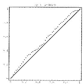
Fig. 2. Q-Q Plots for predictions of individual ship-days.


The second diagnostic check consists in a predictive check of model fit. In particular, we base the posterior analysis on 75% of the entire sample and retain the other 25% for comparison with the corresponding predictive distributions. For all the retained positive observations we record in which percentile of the continuous part of the predictive distributions (based on the inference sample and using the corresponding values of the regressors) the actual observations fall. Contrasting predictive quantiles with empirical ones thus obtained leads to a Q-Q plot that indicates how well the model (estimated on the basis of the inference sample) fits the data in the prediction sample. As the assignment of observations to either sample is random, we would expect such plots to be a good measure of model accuracy. Figure 2 presents these Q-Q plots for all five species, indicating that model fit is always quite adequate. In particular, Species 4 and 5 (grenadier and skate) are very well modeled by this predictive criterion. In the sequel, we shall focus mainly on results for these two species, as well as on Species 2 (halibut), which contributes most to the overall catch, both in weight and in frequency (see Table 2).
5.2. Posterior Results
Here we shall present some results based on the 75% inference sample mentioned above. For policy purposes, the most interesting parameters are the regression coefficients in . In view of space restrictions, we shall limit ourselves to some of the more salient findings. Figures 3-5 present, for a number of selected 's, the posterior p.d.f. in (4.5). In addition, the gauge on top (black shading) indicates the probability that [i.e., with defined just above (4.4)].


Fig. 3. Fishing techniques and net size.


Figure 3 focuses on the effect of fishing techniques and net size. For grenadier the variable ‘drift gillnet’ is often not included in the model (it is, e.g., not in the “best” model), while ‘otter trawl’ is often excluded for skate. For catching grenadier anchored gillnet seems to be the best technique, whereas skate is best caught with an otter trawl or otter trawl by pair (the reference case, as indicated in Table 1). Median catch of skate with an anchored gillnet is only about 1-15% of the median catch with a trawl. In view of the shape of the fish involved, this large difference in the effect of different nets is not too surprising. The influence of net size is also very different for these two species. For grenadier, the elasticity is negative (increasing net size by 1% decreases median catch by 2-6%), whereas for skate there is a positive effect. The latter might indicate that fishing for skate (a relatively broad fish) is typically done with large mesh nets, possibly to avoid too much bycatch.
Some ship characteristics are examined in Figure 4. Spanish vessels are catching more halibut than Portuguese ones (the reference case), whereas the latter seem more successful in the catch of skate. This might simply reflect different target species of these fleets. Vessel length and gross registered tonnage (GRT) are obviously positively correlated measures of the ship's size. For grenadier we mainly include GRT whereas the important “size” variable for skate is the length of the vessel. Another important characteristic of the ship is the power of the engine. As Figure 4 indicates, there is a clear positive effect for the quantity of halibut caught, whereas a negative influence on the catch of skate is inferred. This indicates that more powerful ships will go for the large quantities of halibut, whereas skate (which is usually caught in much smaller quantities per tow; the average positive catch per day is 1,116 kg versus 4,291 kg for halibut) is targeted by the less powerful vessels.

Fig. 5. Zone and Month.

Figure 5 highlights some findings regarding zone and month. For halibut zone 3L seems a much richer part of the fishing ground than the reference zone 3O. However, for skate the best models do not distinguish zones 3L and 3O, and the models that do include 3L indicate that it is even slightly worse than the reference zone. The months of March, May and June are relatively good months for skate (with respect to December), whereas they are much less beneficial to the catch of halibut. Note also that the posterior densities for these months are all bimodal for skate, indicating that some models suggest the influence of these months is much less positive.
5.3. Predictive Results
On the basis of the posterior results partially described above, we shall now predict observations in the 25% of the sample that was not used for posterior inference. Section 5.1 presented Q-Q plots, where predictive and empirical quantiles are contrasted. As examples, we now show some predictive distributions for particular observations in the retained sample.

Fig. 6. Halibut: Predictive densities and actual observed values.

For halibut we can easily compute that the catch is forecasted to be zero with probability 0.185 (from (4.7)), whereas with probability 0.815 it will have a continuous distribution with p.d.f. as in (4.9). Figure 6 shows two such p.d.f.'s for particular values of , along with the actual observation. Observation number i = 1009 (of the 1400 retained observations) corresponds to a fairly large ship in zone 3L, and we see that the actual catch of 6160 kg is well inside the bulk of the predictive mass. Predictive uncertainty, however, is quite substantial. A smaller ship in the somewhat poorer zone 3M (observation 814) will generate more predictive mass on smaller values of , and again the observed value of 1944 kg is very compatible with this predictive distribution.

Fig. 7. Grenadier: Predictive densities and actual observed values.

Some predictive densities for grenadier are presented in Figure 7. Here and i = 375 is a relatively large vessel, fishing in the rather good month of February (actual catch was 380 kg), whereas observation 558 corresponds to a small ship fishing in the worse month of September, catching a mere 75 kg of grenadier. Again, the quantities caught are well matched by the corresponding predictive distributions.

Fig. 8. Skate: Predictive densities and actual observed values.

For skate the predictive probability of zero catch is 0.551 and Figure 8 graphs the p.d.f.'s of the nonzero catch for observations i = 538 and i = 106. Here the crucial importance of the fishing technique is illustrated. Even though observation 106 corresponds to a ship of comparable size to that for i = 538, it uses a drift gillnet and is thus not targeting skate. The very small amount caught (15 kg) is just bycatch. Nevertheless, the predictive distribution captures this feature perfectly. The other ship, using an otter trawl, has a substantial catch (2350 kg) which is well inside the area of predictive mass in Figure 8.
These (arbitrarily chosen) examples illustrate that predictive behaviour is not merely adequate at the aggregate level (as in Subsection 5.1), but leads to useful and reasonable forecasts of the catch of a particular ship, in particular circumstances.


Fig. 9. Q-Q plots for cluster predictions.

For policy purposes, it might be interesting to predict not the catch of one single ship, but the aggregate catch of a number of ships, that are known to be in a certain area of the Grand Bank at a certain time of the year. If we group the data into clusters of 10 observations, we can analyze how such predictions, based on 75% of the observations compare with the actual retained clusters. Clusters of ships that are in the same zone at the same day are likely to be of most interest for practically relevant predictions. In order to mimic such clusters, we have sorted the prediction sample by year, day and zone (in that order) and selected clusters of 10 consecutive observations from that ordering. The procedure outlined in
Subsection 4.2 now leads to the Q-Q plots shown in Figure 9 for Species 2, 4 and 5. These plots indicate that quite adequate predictions can be made for the catch of a certain species aggregated over clusters.


Fig. 10. Predictive densities and actual observed values for clusters.

Figure 10 presents some individual group predictives for the catch of Species 2, 4 and 5. As is to be expected the predictives tend to be more alike across clusters than across single observations, and thus we only present one cluster per species.
6. CONCLUDING REMARKS
In this paper we have outlined the modelling of daily live weight catch of different species of fish in the Grand Banks fisheries. An important aspect of the data is the fact that most days not all species are caught by a certain ship. Thus, modelling of these implicit zero observations is crucial. For the positive observations, we have used a Lognormal regression model, for which we have a collection of 23 different explanatory variables. In order to deal with the 8.4 million possible models that are generated by this, we use Bayesian model averaging. In particular, we apply the MC algorithm of Madigan and York (1995), described for regression models in Raftery et al. (1997). We use a carefully chosen prior distribution and examine posterior and predictive inference. The former can be instrumental in policy decisions regarding the effect of certain ship characteristics or regulations concerning, e.g., net size or fishing techniques. The latter is required if we wish to predict catch per species from easily obtained information regarding the presence of vessels with known characteristics in a certain area at a certain time, rather than having to board these vessels and inspect the catch (which is much more costly and also interferes with the operation of the fishing vessels). Bayesian model averaging naturally takes into account all uncertainty concerning parameter values as well as the model uncertainty (within the class of models considered). Thus, realistic predictions can be made for one or more ship-days, duly taking into account the ships' characteristics, location, month as well as parameter and model uncertainty. Since the programs used were coded efficiently, new data can easily be processed and posterior and predictive inference can be conducted without excessive computational requirements. We have built in two main diagnostic checks that would indicate to the user less thrustworthy results (either because the Markov chain has not yet converged or the particular data are simply not well modelled). Thus, we hope this methodology could contribute to the toolbox of the applied modeller of fish catches.
There are a number of ways in which the sampling model used here could be extended. Firstly, the probability of zero catch, , could be made dependent on certain explanatory variables, such as zone or season, or even perhaps on some characteristics of the fishing vessel. This can easily be implemented without complicating the model substantially. We have experimented with specific 's for each zone-month and found that no substantive improvements in predictive model fit resulted. Therefore, we have opted for the simpler specification used here. A second possible elaboration would be to include ship effects in the continuous part of the model. That could pick up certain quality aspects of the vessels, not captured in the data, but would make prediction for as yet unobserved ships quite difficult. Thirdly, it might be a useful exercise to examine the effects of allowing for heteroskedasticity in the error term of (3.2) by making depend on, e.g., the size of the ship. Of course, both theory and practical implementation would become more cumbersome as a consequence (unless such dependence would be fixed, rather than estimated from the data). Finally, at a considerable cost in terms of added complexity, one might propose a multivariate model for all species with correlated error terms.
References
- FAO (1995), "The State of world fisheries and aquaculture," Rome: United Nations Press.
- Fernández, C., Ley, E. and Steel, M.F.J. (1997), “Benchmark priors for Bayesian Model Averaging,” mimeo, Tilburg University, the Netherlands, Dept. of Econometrics.
- Ferreira, E. and Tusell, F. (1996), “Un modelo aditivo semiparamétrico para estimación de capturas: El caso de las pesquerías de Terranova,” Investigaciones Económicas, 20, 143-157.
- George, E.I. and McCulloch, R.E. (1993), “Variable selection via Gibbs sampling,” Journal of the American Statistical Association, 88, 881-889.
- Hardin, G. (1968), “The tragedy of the Commons,” Science, 162, 1243–1248.
- Hilborn, R. and Walters, C.J. (1992), Quantitative Fisheries Stock Assessment: Choice, Dynamics and Uncertainty, New York: Chapman and Hall.
- Laud, P.W. and Ibrahim J.G. (1995), “Predictive model selection,” Journal of the Royal Statistical Society, B, 57, 247-262.
- Lee, H. (1996), “Model selection for consumer loan application data,” Technical Report 650, Carnegie-Mellon University, Dept. of Statistics.
- Madigan, D. and Raftery, A.E. (1994), “Model selection and accounting for model uncertainty in graphical models using Occam’s Window,” Journal of the American Statistical Association, 89, 1535-1546.
- Madigan, D. and York, J. (1995), “Bayesian graphical models for discrete data,” International Statistical Review, 63, 215-232.
- Min, C. and Zellner, A. (1993), “Bayesian and non-Bayesian methods for combining models and forecasts with applications to forecasting international growth rates,” Journal of Econometrics, 56, 89-118.
- Osiewalski, J. and Steel, M.F.J. (1993), “Regression models under competing covariance structures: a Bayesian perspective,” Annales d’Économie et de Statistique, 32, 65-79.
- Raftery, A.E., Madigan, D. and Hoeting, J.A. (1997), “Bayesian model averaging for linear regression models,” Journal of the American Statistical Association, 92, 179-191.
- Tibbets, J. (1994), “Ocean Commotion,” Environmental Health Perspectives, 104:4, 380–385.
- Zellner, A. (1986), “On assessing prior distributions and Bayesian regression analysis with g-prior distributions,” in: Bayesian Inference and Decision Techniques - Essays in Honor of Bruno de Finetti, eds. P.K. Goel and A. Zellner, Amsterdam: North-Holland, pp. 233-243.
COLECCION RESUMENES
97-01: “Geografía económica y crecimiento”, Juan J. de Lucio.
TEXTOS EXPRESS
97-02: "Il Encuesta sobre la UEM InterMoney-FEDEA: Resultados", C. Arenillas, J. A. Herce, J. A. Ketterer, S. Sosvilla y D. Vegara.
97-01: “La cuestión de las pensiones”, José A. Herce.
DOCUMENTOS DE TRABAJO
97-25: "Statistical modeling of fishing activities in the North Atlantic", C. Fernández, E. Ley y F. J. Steel.
97-24: "Asymmetry in the EMS: New evidence based on non-linear forecasts", O. Bajo-Rubio, S. Sosvilla-Rivero y F. Fernández-Rodríguez.
97-23: “Life expectancy and endogenous growth”, David de la Croix y Omar Licandro.
97-22: “Los efectos de los planes Renove y Prever sobre el reemplazo de turismos”, Omar Licandro y Antonio R. Sampayo.
97-21: “Geografía Económica: Aglomeración, localización y externalidades”, Juan J. de Lucio.
97-20: “Divide et impera: Bargaining and incentives within a hierarchy”, Diego R. Palenzuela y Justo Jorge Moreno.
97-19: “Union effects and the reform of labor relations, with consensus”, Diego R. Palenzuela.
97-18: "Pay determination in the Spanish public sector", Cecilia Albert, Juan F. Jimeno y Gloria Moreno.
97-17: "Provision of private health insurance under public insurance captivity", Diego R. Palenzuela.
97-16: "Inversión directa extranjera y especialización comercial en los países periféricos, Salvador Barrios.
97-15: “Replacement echoes in durable goods purchases”, Raouf Boucekkine y Omar Licandro.
97-14: “Credibility in the EMS: New evidence using nonlinear forecastability tests”, F. Fernández-Rodríguez, S. Sosvilla-Rivero, J. Martín-González.
97-13: “Replacement investment, endogenous fluctuations and the dynamics of job creation and job destruction”, Raouf Boucekkine, Fernando del Rio y Omar Licandro.
97-12: “La demanda de automóviles en España: Un análisis de la evolución y variabilidad de las tasas de reemplazo”, Omar Licandro, Antonio R. Sampayo.
97-11: “Respuesta de los tipos de interés nominales españoles a shocks de inflación esperada y de tipos de interés real ex-ante: Una aplicación VAR estructural”, Vicente Esteve.
97-10: “Convergence in fiscal pressure across EU countries”, Vicente Esteve, Simón Sosvilla y Cecilio Tamarit.
97-09: “Evaluación de los efectos macroeconómicos del fondo de cohesión en España”, Juan Carlos Císcar.
97-08: “Creative destruction, investment volatility, and the average age of capital”, R. Boucekkine, M. Germain, O. Licandro y A. Magnus.
97-07: "Spatially and intertemporally efficient waste management: The costs of interstate flow control", Eduardo Ley, Molly K. Macauley y Stephen W. Salant.
97-06: “Are there any special features in the Spanish business cycle?, Luis Puch y Omar Licandro.
97-05: “Los factores específicos del paro en Andalucía” Juan F. Jimeno.
97-04: “The effects of minimum bargained wages on earnings: Evidence from Spain”, Juan J. Dolado, Florentino Felgueroso y Juan F. Jimeno.
97-03: “Convergence in social protection benefits across EU countries”, Javier Alonso, Miguel Angel
Este texto se ha extraído automáticamente del documento original. Para citarlo o leerlo con su maquetación, descargue el PDF.
Descargar en PDF