HVWXGLRV VREUH OD HFRQRPLD HVSDÔROD
2Q WKH VRXUFHV RI FRQYHUJHQFH $ FORVH ORRN DW WKH 6SDQLVK UHJLRQV
$QJHO GH OD )XHQWH
(((


http://www.fedea.es/hojas/publicado.html
Angel de la Fuente
Instituto de Análisis Económico (CSIC)
and CEPR
Barcelona, October 1997
Abstract
The dominant view in the recent literature on regional convergence seems to be that the evolution of regional incomes in the industrial countries is characterized by very slow but absolute beta convergence. This process of convergence is seen as reflecting the operation of decreasing returns to scale, and its slowness is interpreted as evidence that the technology is close to exhibiting constant returns to scale in a broad capital aggregate.
In this paper we challenge this view on the basis of an analysis of the Spanish experience (1964-91). We develop and estimate a simple descriptive growth model which allows for factor accumulation, technological diffusion and rate effects from human capital and includes fixed regional effects to allow for unobserved factors. The estimated model is then used to quantify the sources of regional convergence. Our results indicate that technological catch-up, the equalization of educational levels and the redistribution of employment across regions account for most of the observed reduction of regional disparities. We also find that, even after controlling for factor stocks and flows and technological diffusion, there remain very significant cross-regional differences in estimated TFP levels which point to the omission of important variables and to the need for a more disaggregated analysis. Finally, we provide some preliminary evidence of the importance of sectoral factors in explaining the evolution of the regional income distribution.
* I would like to thank Rafael Doménech, Xavier Vives and the participants in the CEPR Workshop on Location and Regional Convergence/Divergence for useful comments and suggestions and J. A. Duro for his competent research assistance. Financial support from the Spanish Ministry of Education (DGICYT grant no. PB95-130) and the European Regional Development Fund (through the research project "Determinants of growth at the regional and national level") is gratefully acknowledged.
Address: Instituto de Análisis Económico, Campus de la Universidad Autónoma de Barcelona, 08193, Bellaterra, Barcelona, Spain.
Tel: 34-3-580-6612. Fax: 34-3-580-1452. E-Mail address: delafuente@cc.uab.es.
Non-technical summary
A host of papers have found a negative partial correlation between output per capita (or per worker) and subsequent growth. The strength of this correlation, which is often taken as a measure of the speed of convergence, varies considerably across papers reflecting differences in specification. Estimates of the rate of convergence obtained with unconditional convergence equations (at the regional level), or controlling for investment rates in physical and human capital (at the national level) are typically quite low and cluster around a central value of 2% per year. Recently, however, a number of authors have obtained much higher estimates of the speed of convergence using more flexible specifications which allow more room for regional or national specificities.
From a theoretical perspective these recent estimates are somewhat problematic. Slow convergence can be given a sensible interpretation within a standard neoclassical model as an indication that the technology displays close to constant returns to scale in a broad capital aggregate which includes cumulative investment in education. Within the same framework, however, very fast convergence either takes us back to the old-fashioned neoclassical model with a narrow interpretation of capital (implying that investment in intangibles is not productive), or cannot be explained at all.
This paper argues that in order to make sense of these recent empirical results we must depart from the standard neoclassical framework and think in terms of a broader model which allows for convergence mechanisms other than diminishing returns. Two such mechanisms come immediately to mind: one is technological diffusion across countries and regions (the so-called catch-up effect), and the second one is the reallocation of resources across sectors. One of the objectives of the paper will be to provide quantitative estimates of the contribution of these forces to observed productivity convergence.
Another important implication of some recent studies is that regions (and probably countries) may be far more different from each other than we suspected up to now. Evidence of this, however, comes mostly from non-structural models which rely on dummy variables to pick up all crossregional differences except for initial income and cannot, therefore, give us any indication of even the proximate sources of what seem to be very subtantial productivity differentials. A second goal of this paper will be to determine the extent to which estimated long-term regional disparities may be explained by the forces identified by a further extension of the standard neoclassical model.
To explore these issues we will use a rather comprehensive data set on output levels and factor stocks for the Spanish regions. Our research strategy will be the following. We start by estimating a non-structural, dummy-variable convergence model similar to the one proposed by Canova and Marcet (1995). While this specification is essentially a black box, it does allow us to estimate the distribution of regional productivities to which the sample may be expected to converge in the long run provided "things remain equal", and the speed of convergence of the regional economies towards their stationary relative productivity levels.
We use the results of this dummy-variable model as a benchmark to evaluate the performance of an aggregate structural model which extends the standard neoclassical model by partially endogenizing the rate of technical progress to allow for technological diffusion and the impact of education on total factor productivity (TFP) growth. We proceed essentially by asking to what extent the introduction of the variables suggested by standard growth theory allows us to fit the data (i.e. to generate convergence rates and sustained productivity differentials comparable to those estimated using the benchmark model) without resorting to the use of regional dummies.
The results of the exercise are mixed. On the positive side, our structural model yields very reasonable estimates of the parameters of the production function and we find evidence of a rapid process of technological diffusion across regions. These findings suggest that a suitably extended aggregate model may provide an adequate framework for a first approximation to the analysis of growth and convergence. On the other hand, a version of the model without fixed regional effects presents large and systematic regional residuals which point to important omitted variables and predicts convergence rates which are much lower than our benchmark estimate.
Both problems can be "fixed" through the introduction of fixed regional effects to capture productivity differentials due to unobserved regional characteristics. This gives us a "hybrid" model which generates conditional convergence at just about the right speed and reproduces almost perfectly the observed pattern of relative productivity growth. This model is used to quantify the contribution to the reduction of regional inequality of technological diffusion and factor accumulation, and to provide an estimate of the amount of long-term inequality which is not explained by either of these factors. Our results indicate that technological catch-up, the equalization of educational levels and the redistribution of employment across regions account for most of the observed reduction of regional disparities. We also find that, even after controlling for factor stocks and flows and technological diffusion, there remain very significant cross-regional differences in estimated TFP levels.
This last finding suggests that there is still a lot to do before we can claim a reasonable understanding of the determinants of regional income. Some of our results seem to indicate that sectoral factors may be responsible for at least part of the unexplained productivity differentials and point towards a more disaggregated analysis as a promising strategy for future research. The last part of the paper provides some preliminary evidence which is consistent with this hypothesis.
1.- Introduction
How well can we explain cross-regional (or cross-national) differences in growth patterns and income levels in terms of a simple aggregate model built around a neoclassical production function? The dominant view in the recent growth literature seems to be that the answer to this question is fairly well -- provided we interpret capital as a broad aggregate comprising cumulative investment in human capital as well as in machinery and equipment.
In this paper we will argue that this conclusion is probably too optimistic, and that it is necessary to go beyond the standard neoclassical model with exogenous technological progress in order to provide a reasonably complete account of growth and the evolution of regional (or national) disparities. In particular, we will provide evidence that technological diffusion across regions and changes in the sectoral structure of employment have played an important role in the convergence process. We will also show that significant regional disparities persist even after controlling for aggregate factor stocks and flows and technological diffusion. Some of these findings suggest that further progress in the analysis of growth and convergence will require the development of more disaggregated models.
To reexamine the question raised at the beginning of this introduction we will use a rather comprehensive data set on output levels and factor stocks for the Spanish regions. Our research strategy will be the following. We will start by estimating a non-structural, dummy-variable convergence model similar to the one proposed by Canova and Marcet (1995). While this model is essentially a black box, it will be a useful benchmark because it allows us to obtain estimates of the long-term distribution of relative regional productivities and of the speed of (conditional) convergence towards this distribution. Next, we develop a "structural " model which extends the one commonly used in the literature by partially endogenizing the rate of technical progress. We then ask how far we can get with the structural model, using as an evaluation criterion its performance relative to that of the benchmark model. The results are mixed. Although our estimates of the structural parameters are quite reasonable, the predicted rate of conditional convergence is too low relative to the benchmark estimate and the model leaves substantial residuals which point to large unexplained regional productivity differentials.
To capture these differentials, we finally estimate a "hybrid" model which introduces fixed effects into our structural specification. This model, which reproduces almost exactly the relative growth performance of the different regions, is used to measure i) the sources of observed productivity convergence and ii) the importance of the unexplained regional effects. The large size of these effects, which measure productivity differentials not explained by differences in aggregate factor stocks, indicates that there is still a lot to do before we can claim a reasonable understanding of the determinants of regional income. Some of our results suggest that a good way to start may be to work with more disaggregated models. Towards the end of the paper, we take a first step in this direction and provide some preliminary evidence that sectoral factors have contributed significantly to regional convergence.
The paper is organized as follows. Section 2 reviews some of the key issues in the empirical growth and convergence literature and relates the present paper to previous work in the field. Section 3 briefly discusses the data set we will use and the main features of the process of regional convergence in Spain. In this section we also present the results of the estimation of the nonstructural benchmark model. Section 4 develops a descriptive growth model which allows for technological diffusion across regions and rate effects from human capital and derives an empirical specification which allows us to estimate technological differentials across regions simultaneously with the coefficients of the production function. Section 5 presents the empirical results and discusses the extent to which the factors included in the model can account for estimated long-term cross-regional productivity differentials and convergence rates. In Section 6 the model is used as a framework for a "convergence accounting" exercise which yields quantitative estimates of the contributions of technological diffusion and factor accumulation to observed productivity convergence. In Section 7 we abandon our aggregate model and report on some preliminary work which suggests that sectoral factors have played an important role in regional convergence. Section 8 concludes with a brief summary.
2.- Some issues in the convergence literature
Following the pioneering work of Barro and Sala i Martin (1990) a large number of authors have investigated the pattern of convergence in different national and regional samples using "structural" convergence equations derived from explicit growth models.1 Several empirical regularities with potentially important theoretical and policy implications have emerged from this work.
First, practically all existing studies find evidence of a negative partial correlation between growth and initial income (i.e. of beta convergence) both at the national and regional levels. At the national level the convergence result is typically of a conditional nature. In broad samples, poorer countries tend to grow faster than richer ones only once we condition on investment in physical and human capital and other variables. At the regional level, however, the consensus view seems to be that convergence is absolute. The correlation between initial income per capita and subsequent growth is typically negative in such samples even without controlling for additional variables. This fact is often interpreted to imply that the regions of the industrial countries tend to converge to a common level of income per capita in the long run.
1 See for example Barro and Sala (1991, 1992a and b), Sala (1995, 1996), Mankiw, Romer and Weil (1992), Shioji (1992), Coulombe and Lee (1993), Dolado et al (1994), Mas et al (1994), Raymond and García (1994) and Mankiw (1995). Antecedents to the work of Barro and Sala may be found in Baumol (1986), Romer (1987) and Dowrick and Nguyen (1989). For a survery of this literature and a more detailed discussion of the issues raised in this section see de la Fuente (1997).
A second key finding is that the speed of convergence seems to be very low but quite stable across samples. Most estimates of the rate of convergence cluster around a central value of 2% per annum. Since this estimate implies that the half-life of the convergence process is around 35 years, the elimination of income disparities would take several decades even if convergence is absolute. The remarkable stability of the convergence coefficient, on the other hand, seems to indicate that the forces behind income convergence operate in a regular fashion across time and space and suggest that this parameter may be given a structural interpretation in terms of a common theoretical model.
The most popular interpretation of the convergence parameter seems to be that it reflects mostly the operation of diminishing returns to scale in reproducible factors. Barro and Sala i Martin (1990, 1992) and Mankiw, Romer and Weil (1992), for example, interpret their empirical results within the framework of a neoclassical model with exogenous technical progress. This allows them to explicitly relate the rate of convergence to the coefficients of the aggregate production function and other structural parameters.2 In this context, the finding of slow convergence must be interpreted as an indication that the technology exhibits almost constant returns to scale in reproducible factors. As Barro and Sala i Martin (1990, 1992) argue, this conclusion seems much more plausible when we think in terms of a broad capital aggregate than when we interpret capital in a restrictive fashion as the sum of the stocks of equipment and structures. Mankiw, Romer and Weil (1992) provide some empirical support for this view using an extension of the Solow model which incorporates human capital as a factor of production.
Aside from the switch to a broader concept of capital, the consensus view which emerges from the work we have briefly reviewed seems to be that a suitably extended version of the basic neoclassical model provides an adequate description of the main forces underlying the convergence process. Some recent empirical papers, however, raise what would seem to be a serious challange to this interpretation. Marcet (1994) and Canova and Marcet (1995), for instance, question the accuracy of previous estimates of the convergence parameter and, indirectly, the conclusion that there exist almost constant returns to scale in reproducible factors. Since it is necessary to know the position of the steady state in order to estimate the speed of convergence with precision, the omission of various determinants of long-run income could bias the estimates of the convergence parameter towards zero in standard growth regressions. To explore this possibility, these authors estimate a Bayesian model with panel data, introducing fixed effects to control for possible differences across territories, and obtain convergence rates which are much higher than those found in other studies (around 11% for a sample of OECD countries and 23% for European regions). In the same line, Raymond and García (1995) obtain comparable convergence rates for the Spanish regions using a fixed-effects model, and Islam (1995) obtains estimates of the rate of convergence ranging between 4.3 and 9.3% using a panel data specification with fixed country effects.
β = (1-α)(δ+g+n)
2 Mankiw, Romer and Weil (1992), for example, show that in the context of the traditional Solow model the rate of convergence is given by , where α is the coefficient of capital in the aggregate production function, g the rate of technical progress, δ the rate of depreciation and n the rate of labour force or population growth.
These papers yield a view of the convergence process which is quite different from the dominant one in the literature, particularly at the regional level. Instead of slow but absolute convergence to a common income level, these studies point to extremely rapid convergence but to very different steady states and, therefore, to the indefinite persistence of large regional disparities. From a theoretical point of view, moreover, these results are hard to reconcile with the extended neoclassical model. When we interpret them in this framework, the new estimates of the convergence rate take us back to the standard Solow model with a narrow definition of capital in the best of cases, and lead to non-sensical results (such as a negative capital coefficient) in many others.
The starting point of this paper is the idea that, in order to make sense of these recent empirical results, we must depart from the standard neoclassical framework and think in terms of a broader model which allows for convergence mechanisms other than diminishing returns. Two such mechanisms come immediately to mind: one is technological diffusion across countries and regions (the so-called catch-up effect), and the second one is the reallocation of resources across sectors. Once we take these factors into account, the estimated speed of convergence (particularly when it comes from an unconditional convergence regression) must be seen as a summary statistic for the net effect of various forces --rather than as an indirect estimate of a parameter of the production function. From this perspective, the findings of Canova and Marcet and other authors indicate that, if we have measured correctly the speed of convergence, the process is much too fast to be explained only in terms of diminishing returns. This suggests that the alternative convergence mechanisms we have just mentioned (and probably others) are more important than we thought previously and deserve far more attention than they have received so far in the literature. One of the objectives of this paper will be to provide quantitative estimates of the contribution of some of these forces to observed productivity convergence.
Another important implication of the results we have just sketched is that regions (and probably countries) may be far more different from each other than we suspected up to now. Evidence of this, however, comes mostly from non-structural models which rely on dummy variables to pick up all cross-regional differences except for initial income and cannot, therefore, give us any indication of even the proximate sources of what seem to be very subtantial productivity differentials. A second goal of this paper will be to determine the extent to which estimated long-term regional disparities may be explained by the forces identified by a further extension of the standard neoclassical model. As may be expected, controlling for factor stocks and flows and for technological diffusion significantly reduces this unexplained component of long-term relative incomes but does not eliminate it. In fact, substantial disparities remain even after controlling for such factors. This refined "residual," in addition to providing a summary measure of the inadequacies of our aggregate model, may also give us some clues about the sorts of things that we should be looking into. Trying to see what is inside this black box is certainly a promising area for future research.
3.- A first look at the Spanish data
In this paper we will use Spain as a sort of laboratory for the analysis of regional convergence. The main reason is that, while Spain presents what seems to be a "representative" convergence pattern, we have access to relatively long and fairly detailed series on regional productivity and factor stocks. The available information includes (mostly) bi-annual series on regional gross value added and employment covering the period 1955-91 with some degree of sectoral disaggregation, and annual series on regional physical capital stocks and investment flows (Fundación BBV, 1996) and on the educational composition of the labour force (Mas et al, 1996) which cover the period from 1964 to 1991.
The income and employment series have been constructed by the research department of a large Spanish bank (Banco Bilbao-Vizcaya, various years), while the data on factor stocks has been assembled by the Instituto Valenciano de Investigaciones Económicas using the Labour Force and Industrial Surveys and various other sources. Most of these figures are estimates based on primary sources of varying coverage and reliability and they are certainly not free of problems. They do, however, have some important advantages: they are carefully constructed and exploit practically all available primary information, and they are fully comparable across regions and over time. On the whole, this is the richest regional data set we are aware of and it does allow an investigation of the sources of growth and convergence at a level of detail which, to our knowledge, would not be possible for any other country, with the possible exception of the U.S.
In this section we will take a preliminary look at the pattern of regional convergence in Spain. As we have anticipated, this pattern seems to be representative of those found in most other industrial countries. The level of regional inequality (measured by the coefficient of variation of log output per employed worker) decreases significantly over the last few decades, although it stabilizes somewhat in the latter part of the period (see Figure 1). As for the pattern of beta convergence, an unconditional regression of average productivity growth rates on the log of initial output per employed worker yields an estimated convergence rate which is not far from the usual 2% (see Figure 2). To give the reader an idea of where each region stands, Figure 3 shows the initial and final position of each of them in terms of its relative productivity, defined as log output per employed worker measured in deviations from its contemporaneous sample average. (Since we will concentrate below on the period 1964-91, most of the information contained in these figures refers to these years).
Figure 1: σ-convergence in productivity among the Spanish regions, 1955-1991 - Note: standard deviation of relative productivity, defined as log output per employed worker expressed in deviations from its sample average.
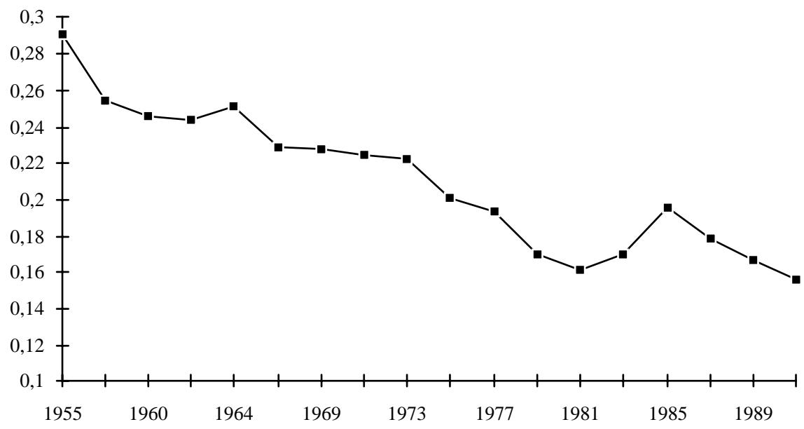
Figure 2: Unconditional beta convergence among the Spanish regions, 1964-91 productivity growth log initial productivity,
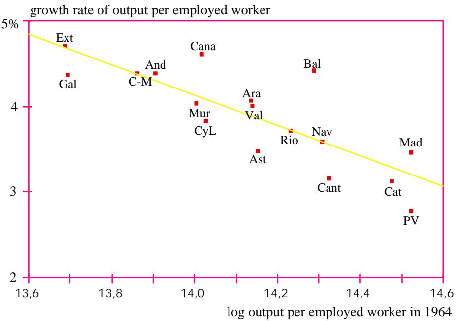
- Legend: Ext = Extremadura, Gal = Galicia, And = Andalucía, C-M = Castilla la Mancha, Cana = Canarias, Mur = Murcia, C-L = Castilla y León, Ara = Aragón, Val = Valencia, Ast = Asturias, Rio = Rioja, Bal = Baleares, Nav = Navarra, Cant = Cantabria, Cat = Cataluña, Mad = Madrid, PV = País Vasco.
Figure 3: Relative productivity in 1964 and 1991
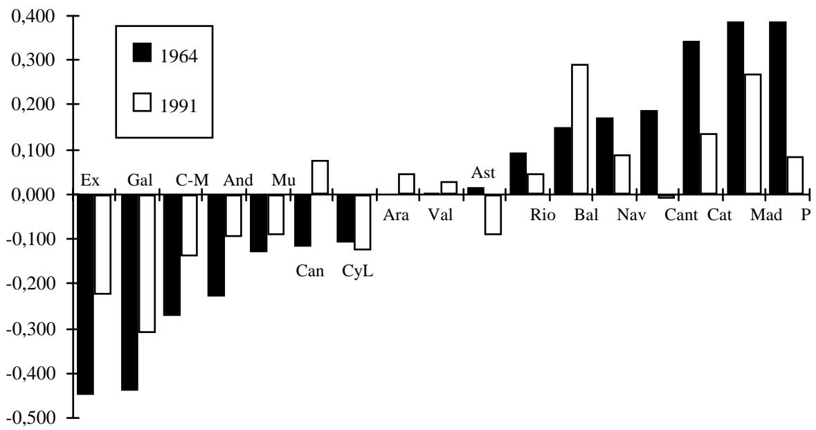
Figure 4: Employment growth vs initial productivity growth of employment = -0.22794 + 0.01604 log initial productivity,
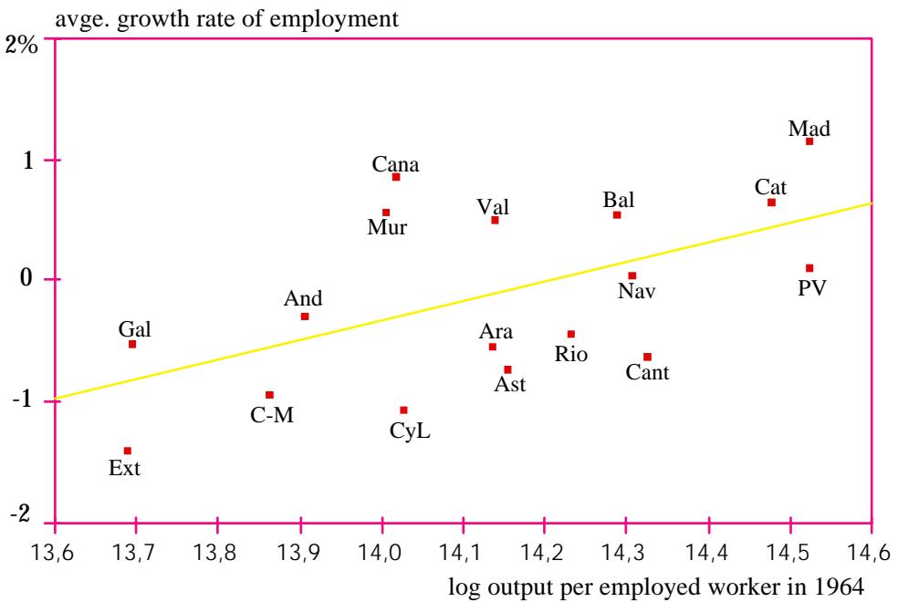
Figure 4 shows that convergence in productivity has been accompanied by an increasing concentration of employment and economic activity in the initially richer regions. Although this fact has not been emphasized in the literature on regional convergence, it too seems to be representative of the experience of a good many countries.
- A benchmark model
As a starting point for our investigation of regional convergence we will estimate a "nonstructural" model which relies on dummy variables to empirically capture the permanent component of cross-regional productivity differentials. The specification we will use is a (non-bayesian) variant of the one proposed by Canova and Marcet (1995).
We will assume that the evolution of relative regional productivity, can be described by an equation of the form
\[\Delta \mathbf {q} _ {\mathbf {i}, t} = \mathbf {x} _ {\mathbf {i}} - \beta \mathbf {q} _ {\mathbf {i}, t} + \varepsilon_ {\mathbf {i} t} \tag {1}\]
where the term is used to capture region-specific effects and is a random disturbance. Iterating (1) backwards we obtain the equation
\[{(2) \frac {\mathbf {q _ {i , t}} - \mathbf {q _ {i , t - h}}}{h} = \frac {1 - \lambda^ {h}}{h} (\mathbf {q _ {i}} ^ {*} - \mathbf {q _ {i , t - h}}) + \mathbf {u _ {i , t , h}}}\]
where and the error term is a weighted average of the annual disturbances,
\[\mathbf {u _ {i , t , h}} = \frac {1}{h} \sum_ {s = 0} ^ {h - 1} \lambda^ {s} \varepsilon_ {i, t - 1 - s}.\]
Equation (2) shows that the growth rate of relative productivity in region i during the period from th to t is a function of the initial deviation of relative productivity from its expected steady-state value, Working with panel data on output per employed worker and introducing regional dummies, we can use NLS to estimate the convergence coefficient, , and the steady-state levels of relative income for the different regions.
Table 1 shows the results obtained with two variants of this specification. Since (the log of) regional productivity is measured in deviations from the average, absolute convergence would imply for all i. In equation [1], where this restriction is imposed ex ante, we obtain a convergence coefficient which, once more, is not very far from the standard 2%. Equation [2] is of the
form
\[\frac {\mathbf {q} _ {\mathrm{i,t}} - \mathbf {q} _ {\mathrm{i,t-h}}}{\mathrm{h}} = \frac {1 - \lambda^ {\mathrm{h}}}{\mathrm{h}} \left(\sum_ {\mathrm{i}} \Gamma_ {\mathrm{i}} \mathrm{DREG} _ {\mathrm{i}} - \mathbf {q} _ {\mathrm{i,t-h}}\right) + \mathbf {u} _ {\mathrm{i,t,h}}.\]
Hence, the coefficient of each of the regional dummies (DREG ) gives us an estimate of the corresponding steady state. We observe that the estimated rate of convergence increases four-fold (from 3% to 12.7%) and that more than half of the regional dummies are significant. The hypothesis of absolute convergence is, therefore, clearly rejected.
Notes:
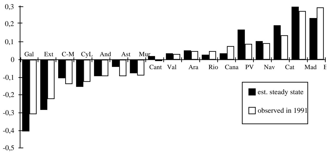
The preceding results (which closely resemble those obtained by Marcet (1994), Canova and Marcet (1995) and Raymond and García (1994) with similar specifications) suggest a vision of the convergence process which is quite different from the one advanced by Barro and Sala i Martin (1990, 1992). In particular, the results of the conditional specification with fixed regional effects point to the possibly indefinite persistence of important regional disparities. As can be seen in the last row of Table 1, the dispersion of estimated long-run relative productivities is quite similar to, and indeed a bit larger than, the dispersion observed in 1991. On the basis of these results, there would be no reason to expect a significant decrease in regional inequality in the future or many changes in the relative position of the different regions. Figure 5, which shows the relative productivity of each region in 1991 along with its estimated steady state, reinforces this message. The Spanish regions seem to be very close to their steady states. 3
Table 1: Productivity convergence among the Spanish regions, 1955-91
| [1] | [2] | |||
| coefficient | (t) | coefficient | (t) | |
| Conv. coeff. (β) | 0.0295 | (4.78) | 0.1273 | (6.23) |
| Madrid | 0.2985 | (6.84) | ||
| Baleares | 0.2344 | (5.36) | ||
| Cataluña | 0.1930 | (4.34) | ||
| País Vasco | 0.1701 | (3.69) | ||
| Navarra | 0.1056 | (2.44) | ||
| Aragón | 0.0500 | (1.15) | ||
| Valencia | 0.0344 | (0.80) | ||
| Canarias | 0.0343 | (0.77) | ||
| Rioja | 0.0289 | (0.67) | ||
| Cantabria | 0.0210 | (0.48) | ||
| Asturias | -0.0404 | (0.92) | ||
| Murcia | -0.0766 | (1.77) | ||
| Andalucía | -0.0938 | (2.16) | ||
| Castilla y León | -0.1067 | (2.47) | ||
| Castilla la Mancha | -0.1554 | (3.54) | ||
| Extremadura | -0.2834 | (6.44) | ||
| Galicia | -0.4036 | (9.24) | ||
| $R^2$ | 0.0758 | 0.1924 | ||
| s.e. of the reg. | 0.0219 | 0.0211 | ||
| std. dev. of $y_i^*$ | 0.1753 | |||
| s. d. of $y_i$ in 1991 | 0.1558 | |||
- Panel estimates with 17 observations per region (corresponding to two or three-year intervals).
R2
3 A regression of the estimated steady state on the observed value of relative productivity in 1991 yields an of 0.94.
- The output variable is (log) output per employed worker, measured in deviations from the sample average in each period.
Figure 5: Relative productivity, observed value in 1991 vs. estimated long-run level
What should we make of estimates of the rate of convergence as different from each other as those given in equations [1] and [2] of Table 1? If we want to give this parameter a structural interpretation in terms of capital's coefficient in the production function, equation [1] is probably misspecified and should be ignored. This first estimate, however, can still be of considerable interest as a summary mesure of the net strength of the tendency towards the reduction of inequalities. The second estimate, on the other hand, would provide a better measure of the speed at which each region approaches its position in a stationary distribution characterized by a considerable amount of regional inequality.4 Although this conditional convergence rate is (hopefully) susceptible of a structural interpretation, an estimate exceeding 12% cannot be explained in terms of the standard neoclassical model. To see this, notice that if we interpret the estimated value of β within the framework of the Solow model with exogenous technological progress, this parameter will be related to the coefficient of capital in the aggregate production function by the expression (see footnote 2):
4 When we speak about the speed of convergence it is important to specify the "target point" with respect to which we are measuring convergence rates. It must also be recognized that all such points are merely hypothetical in the sense that there is no way to ensure that the system is actually converging towards them. In equation [2] the target is an estimated asymptotic distribution of regional productivities, but this distribution will only be attained if "nothing changes." In equation [1] the target is a sigle point. If equation [2] describes the correct model, such a point will never be attained, but it is still useful to measure the rate at which the system is closing the gap with respect to it.
\[\alpha = 1 - \frac {\beta}{\mathbf {g} + \mathbf {n} + \delta},\]
where the denominator is the sum of the rates of technical progress (g), employment growth (n) and depreciation (δ). If we assume a value of 2% of g and use the average values of n and δ in our data (see Section 5 below), the implied value of α is -1.05. Since a negative capital coefficient makes no sense, we should take this result as a clear indication that forces other than decreasing returns must be contributing to (conditional) convergence.
One of the key objectives of this paper will be to explore the role of two such forces. Working within a highly aggregated model we will first analyze the contribution of technological diffusion to regional convergence. The same model will also be used to investigate what lies behind the longterm disparities captured by the fixed effects. The two main tests to which we will put this model are its ability to i) generate rates of convergence comparable to the one we have just estimated and ii) reduce the size of the unexplained productivity differentials captured by the regional dummies. Towards the end of the paper, we will turn to the role of sectoral factors in convergence.
4.- A framework for empirical analysis
Our first look at the data is quite consistent with the results of previous studies. Unconditional convergence regressions yield a value of beta close to the ubiquitous 2%, while a specification with fixed regional effects suggests much faster convergence but to very different steady states. One thing the dummies cannot do for us, however, is tell us what forces have generated the observed degree of convergence or what factors explain the persistent disparities we find across regions. To explore these issues we will begin by developing a simple empirical model by augmenting a standard aggregate production function with a technical progress function which allows for technological diffusion and rate effects from human capital. We will also leave room for unobserved fixed regional effects by postulating that TFP levels may differ across regions due to specific, "non-transferrable" factors. The model is similar to the one developed by de la Fuente (1995). The main difference has to do with the model's empirical implementation: since we have data on factor stocks we can estimate the production function directly -- rather than resort to the usual log-linear approximation in order to work with data on investment flows.
Following the standard practice in the literature, we will assume a Cobb-Douglas aggregate production function of the form
\[(3) \mathrm{Y} _ {\mathrm{it}} = \mathrm{K} _ {\mathrm{it}} ^ {\theta \mathrm{k}} (\mathrm{R} _ {\mathrm{i}} \mathrm{A} _ {\mathrm{it}} \mathrm{L} _ {\mathrm{it}}) ^ {\gamma} (\mathrm{R} _ {\mathrm{i}} \mathrm{A} _ {\mathrm{it}} \mathrm{L} _ {\mathrm{it}} \mathrm{H} _ {\mathrm{it}}) ^ {\eta} = \mathrm{K} _ {\mathrm{it}} ^ {\theta \mathrm{k}} (\mathrm{R} _ {\mathrm{i}} \mathrm{A} _ {\mathrm{it}} \mathrm{L} _ {\mathrm{it}}) ^ {\theta \mathrm{l}} \mathrm{H} _ {\mathrm{it}} ^ {\theta \mathrm{h}}\]
where and In this expression Y denotes aggregate regional output, K the (private) stock of physical capital, L is employment and H an indicator of the stock of human capital per worker. The main difference with standard specifications is that we will assume that the index of regional technical efficiency has two distinct components, and . We will interpret the first one, as an index of "transferable" technical knowledge, and the second one, as a term which captures specific and non-transferable regional characteristics which may have an impact on productivity (e.g. geographic location, climate, endowment of natural resources and other determinants of a region's pattern of comparative advantage).
Taking logarithms of this expression (denoted by lower-case letters) and adding the rate of unemployment, u, to control for cyclical shocks, we obtain
\[\mathbf {y} _ {\mathrm{it}} = \theta_ {\mathrm{l}} \mathbf {r} _ {\mathrm{i}} + \theta_ {\mathrm{l}} \mathbf {a} _ {\mathrm{it}} + \theta_ {\mathrm{k}} \mathbf {k} _ {\mathrm{it}} + \theta_ {\mathrm{l}} \mathbf {l} _ {\mathrm{it}} + \theta_ {\mathrm{h}} \mathbf {h} _ {\mathrm{it}} + \theta_ {\mathrm{u}} \mathbf {u} _ {\mathrm{it}}. \tag {4}\]
Taking differences of this expression and adding a random disturbance, (ωit), the equation to be estimated is of the form:
\[\Delta \mathbf {y} _ {\mathrm{it}} = \theta_ {\mathrm{l}} \Delta \mathbf {a} _ {\mathrm{it}} + \theta_ {\mathrm{k}} \Delta \mathbf {k} _ {\mathrm{it}} + \theta_ {\mathrm{l}} \Delta \mathbf {l} _ {\mathrm{it}} + \theta_ {\mathrm{h}} \Delta \mathbf {h} _ {\mathrm{it}} + \theta_ {\mathrm{u}} \Delta \mathbf {u} _ {\mathrm{it}} + \omega_ {\mathrm{it}}.\]
To complete the specification we will partially endogenize the rate of technical progress, writing it as a function of the stock of human capital per worker and the technological gap between each region and a national average. We will start by writing the (log of the) level of transferable technical efficiency of region i at time t in the form
\[\mathbf {a _ {i t}} = \mathbf {a _ {t}} + \mathbf {d _ {i t}} \tag {6}\]
where is the "national average" of and the "tecnological distance" between region i and the average. In what follows, we will treat the average level of (transferable) technical efficiency, , as an exogenous variable (possibly determined by the technological gap between Spain and other countries and the level of R&D effort) and focus on the determinants of the evolution of the relative technical efficiency of each region.
In particular, we will assume that
\[(7) \Delta \mathbf {a} _ {\mathbf {t}} = \mathbf {g} + \mathbf {c t},\]
i.e. that the average rate of technical progress is equal to an exogenous constant plus, possibly, a trend, and that the technological differential of region i evolves following the equation5
\[(8) \Delta \mathrm{d} _ {\mathrm{it}} = \mu \widetilde {\mathrm{h}} _ {\mathrm{it}} - \varepsilon \mathrm{d} _ {\mathrm{it}}\]
where h is the stock of human capital per worker in region i measured in differences with the national average, . The technical progress differential in favour of a given region depends, therefore, on two factors: its relative educational level and its (transferable) technological gap relative to the average region. If there is a process of technological diffusion across regions (that is, if the more backwards regions enjoy the advantage of being able to adopt at low cost the technologies used in the more advanced ones), the coefficient of should be negative -- that is, other things equal, the rate of technical progress should be higher in the less developed regions. The sign of the coefficient ε will therefore allow us to test the hypothesis that there is a process of technological convergence across regions. is different from zero, such convergence would only be conditional, with each region converging in the long run (given a constant value of to a stable level of relative technical efficiency which would be determined by the educational level of its labour force and the speed of technological diffusion, ε.
5 If we were working with national data it would be both possible and desirable to include in the equation some indicator of R&D investment as a determinant of the rate of technical progress. At the regional level, however, we lack detailed data on the distribution of R&D expenditures. The available information suggests that R&D investment is heavily concentrated in Madrid, Catalonia and the Basque Country. On the other hand, many firms whose research labs are located in these regions have productive facilities throughout the country which would also benefit directly from this research. Hence, it may not be a good idea to try to regionalize R&D expenditures, even if sufficient information were available to do so.
Adding (7) and (8), the rate of techical progress in region i during period t will be given by:
\[(9) \Delta \mathbf {a _ {i t}} = \Delta \mathbf {a _ {t}} + \Delta \mathbf {d _ {i t}} = \mathbf {g} + \mathbf {c t} + \mu \widetilde {\mathbf {h _ {i t}}} - \varepsilon \mathbf {d _ {i t}}.\]
Substituting this expression into (5) we obtain a specification of the production function in first differences in which the rate of technical progress is expressed as a function of the relative educational level of each region and its technological gap with respect to an average region.
In order to estimate equation (9) we have to find some way of measuring the transferable technological gap, dit. This variable is not directly observable in principle but, since we have data on factor stocks and regional incomes, we can invert the production function and write as a function of observable variables and coefficients to be estimated. In particular, solving for ait in (4) and ignoring the disturbance we have:
\[\mathrm{a} _ {\mathrm{it}} = \frac {\mathrm{y} _ {\mathrm{it}} - \theta_ {\mathrm{k}} \mathrm{k} _ {\mathrm{it}} - \theta_ {\mathrm{l}} \mathrm{l} _ {\mathrm{it}} - \theta_ {\mathrm{h}} \mathrm{h} _ {\mathrm{it}} - \theta_ {\mathrm{u}} \mathrm{u} _ {\mathrm{it}} - \theta_ {\mathrm{l}} \mathrm{r} _ {\mathrm{i}}}{\theta_ {\mathrm{l}}} . \tag {10}\]
Since the equation is linear in logs, moreover, the same relation will hold among the averages of the relevant variables. This allows us to compute at using
\[(1 1) a _ {t} = \frac {y _ {t} - \theta_ {k} k _ {t} - \theta_ {l} l _ {t} - \theta_ {h} h _ {t} - \theta_ {u} u _ {t} - \theta_ {l} r}{\theta_ {l}},\]
where the absence of the subindex i indicates that we are working with interregional averages (of the variables in logs). Subtracting (11) from (10), the transferable technological gap of region i relative to the average at time t will be given by:
\[\mathrm{d} _ {\mathrm{it}} = \widetilde {\mathrm{a}} _ {\mathrm{it}} = \mathrm{a} _ {\mathrm{it}} - \mathrm{a} _ {\mathrm{t}} = \frac {\widetilde {\mathrm{y}} _ {\mathrm{it}} - \theta_ {\mathrm{k}} \widetilde {\mathrm{k}} _ {\mathrm{it}} - \theta_ {\mathrm{l}} \widetilde {\mathrm{l}} _ {\mathrm{it}} - \theta_ {\mathrm{h}} \widetilde {\mathrm{h}} _ {\mathrm{it}} - \theta_ {\mathrm{u}} \widetilde {\mathrm{u}} _ {\mathrm{it}} - \theta_ {\mathrm{l}} \widetilde {\mathrm{r}} _ {\mathrm{i}}}{\theta_ {\mathrm{l}}} \tag {13}\]
where the tildes denote deviations from the regional average and, in particular, , with
Combining (13) with the previous expressions and introducing dummy variables (DREGi) to capture the fixed regional effects, ri, we finally arrive at a specification written entirely in terms of observable variables and coefficients to be estimated:
\[\begin{array}{l} \text {(14)} \Delta \mathrm{y} _ {\mathrm{it}} = \theta_ {\mathrm{l}} (\mathrm{g} + \varepsilon \widetilde {\mathrm{r}} _ {\mathrm{v}}) + \theta_ {\mathrm{l}} \mathrm{ct} + \theta_ {\mathrm{k}} \Delta \mathrm{k} _ {\mathrm{it}} + \theta_ {\mathrm{l}} \Delta \mathrm{l} _ {\mathrm{it}} + \theta_ {\mathrm{h}} \Delta \mathrm{h} _ {\mathrm{it}} + \theta_ {\mathrm{u}} \Delta \mathrm{u} _ {\mathrm{it}} + \\ \qquad + \theta_ {\mathrm{l}} \mu \widetilde {\mathrm{h}} _ {\mathrm{it}} - \varepsilon \left(\widetilde {\mathrm{y}} _ {\mathrm{it}} - \theta_ {\mathrm{k}} \widetilde {\mathrm{k}} _ {\mathrm{it}} - \theta_ {\mathrm{l}} \widetilde {\mathrm{l}} _ {\mathrm{it}} - \theta_ {\mathrm{h}} \widetilde {\mathrm{h}} _ {\mathrm{it}} - \theta_ {\mathrm{u}} \widetilde {\mathrm{u}} _ {\mathrm{it}} - \sum_ {\mathrm{i} \neq \mathrm{v}} \Gamma_ {\mathrm{i}} D R E G _ {\mathrm{i}}\right) + \omega_ {\mathrm{it}}. \end{array}\]
where the subindex v denotes a reference region and the coefficient of the i-th regional dummy is of the form
5.- Empirical results and the extent of unexplained long-term disparities
In this section we present the results of the estimation of different variants of equation (14) using panel data for the Spanish regions for the period 1964-1991. Since our output series is (mostly) biannual, we are limited to 13 observations per region. Our proxy for the stock of human capital per worker is the fraction of the employed population which have at least some secondary schooling. Table 2 gives the definition and sources of the different variables used in the analysis.
Table 2: Definition and sources of the variables
| yit = logarithm of regional output (gross value added) in millions of 1990 pesetas. Source: Banco Bilbao-Vizcaya (various years). |
| lit = logarithm of total employment in region i at time t (average over the four quarters). Source: Banco Bilbao-Vizcaya (various years). |
| kit = logarithm of the net stock of privately held physical capital in region i at time t, in millions of 1990 pesetas, computed as the average of the beginning and end-of-year stocks (except for the first year in the sample). Source: Fundación BBV (1996). |
| hit = logarithm of the fraction of the employed population (in region i at time t) which has at least started (but not necessarily completed) secondary schooling. The figure includes workers who have started higher levels of education. Source: Mas et al (1995). |
| uit = average rate of unemployment. Source: Mas et al (1995) from the Labour Force Survey. |
| Δxit = (xi,t+h - xi,t)/h = average growth rate of the variable X (= Y, K, L, A...) during the subperiod from t to t+h. |
r∼ v ≅ 0
6 In the following section we will select the reference region so that and ignore this term most of the time. The exception will be the "convergence accounting" exercise of Section 6, where we will attribute to a hypothetical average region the computed average of the coefficients of the dummies and express those of each of the 17 regions in deviations from this figure. This procedure gives the reference region (Valencia) a value of θlrv equal to 0.0043.
We will start by estimating equation (14) without fixed regional effects (i.e. after imposing the assumption that for all i). Table 3 shows the results obtained with different variants of this specification. In equation [3] we impose the assumption that the rate of technical progress is exogenous and common to all the regions . The coefficient of physical capital in this specification is very low (0.154) and insignificant at 5% while the coefficients of the other productive factors are significant and have reasonable values. In equation [4] we introduce a technological diffusion effect while maintaining the assumption that the rate of technical progress is independent of the level of schooling of the workforce . The coefficient which captures technological diffusion is positive and significant, although relatively small (2.7% per year). On the other hand, the coefficient of physical capital becomes significant in this equation and is close to the expected value of one third (capital's share in national income), while the coefficients of human capital and labour maintain their significance and their reasonable values.
In equation [5] we allow the rate of technical progress to be a function of the relative educational level of each region, thus introducing a "rate effect" of human capital (in addition to the "level effect" captured by . The coefficient which captures this new effect is positive and significant. As for the rest of the regressors, the estimated value of the rate of technological convergence increases by a factor of 2.5 (from 2.7 to 6.6%) while the coefficients of the factor stocks remain stable with a slight increase in the precision of the estimates. Since the sum of the relevant parameters is not significantly different from 1, in equation [6] we impose the assumption of constant returns to scale in labour and physical and human capital (that is, , obtaining results which are very similar to those obtained with the previous specification.7 Of particular interest is the fact that our estimate of ε suggests that the rapid (conditional) convergence of total factor productivity levels across regions may be more important as a source of productivity convergence than the operation of decreasing returns.
7 Equations [4]-[6] are estimated using an iterative NLS algorithm which starts from given initial values of the parameters. It must be observed that the results are sensitive to the choice of initial values. If we start from the values of the parameters of the production function estimated in [3] and zero initial values of µθl and ε, the μθ1 algorithm converges to values which are very close to the initial ones. The results shown in the table are obtained starting from positive values of the last two coefficients and a value of for θk. The resulting 1/3 θk. estimates, besides being more reasonable, yield a higher value of the likelihood function and a higher R2, although the difference in this respect between the two sets of estimates is small.
Table 3: Results without fixed regional effects
| [3] | [4] | [5] | [6] | |
| $\theta_k$ | 0.1542(1.76) | 0.3014(4.24) | 0.3419(5.56) | 0.3518(6.18) |
| $\theta_l$ | 0.5396(7.79) | 0.6521(10.97) | 0.6471(11.36) | [0.6482] |
| $\theta_h$ | 0.1830(3.48) | 0.1728(3.17) | 0.1773(3.28) | 0.1767(3.28) |
| $\theta_u$ | -0.1679(1.06) | 0.0459(0.33) | 0.0294(0.22) | 0.0301(0.23) |
| $g\theta_l$ | 0.0326(4.39) | 0.0235(3.44) | 0.02053(3.21) | 0.0199(3.20) |
| $c\theta_l$ | -0.00106(4.18) | -0.00086(3.49) | -0.00078(3.28) | -0.00076(3.26) |
| ε | [0.00] | 0.0272(2.20) | 0.06656(3.55) | 0.06765(3.63) |
| $μ\theta_l$ | [0.00] | [0.00] | 0.0201(2.42) | 0.0201(2.44) |
| $R^2$ | 0.4482 | 0.4486 | 0.4634 | 0.4629 |
| std. error | 0.02177 | 0.02182 | 0.02157 | 0.02153 |
Notes: - t statistics shown in parentheses below each coefficient. - The coefficients which appear in brackets are imposed rather than estimated. In equation [6] the coefficient is estimated after imposing the assumption that The value of shown in the table is
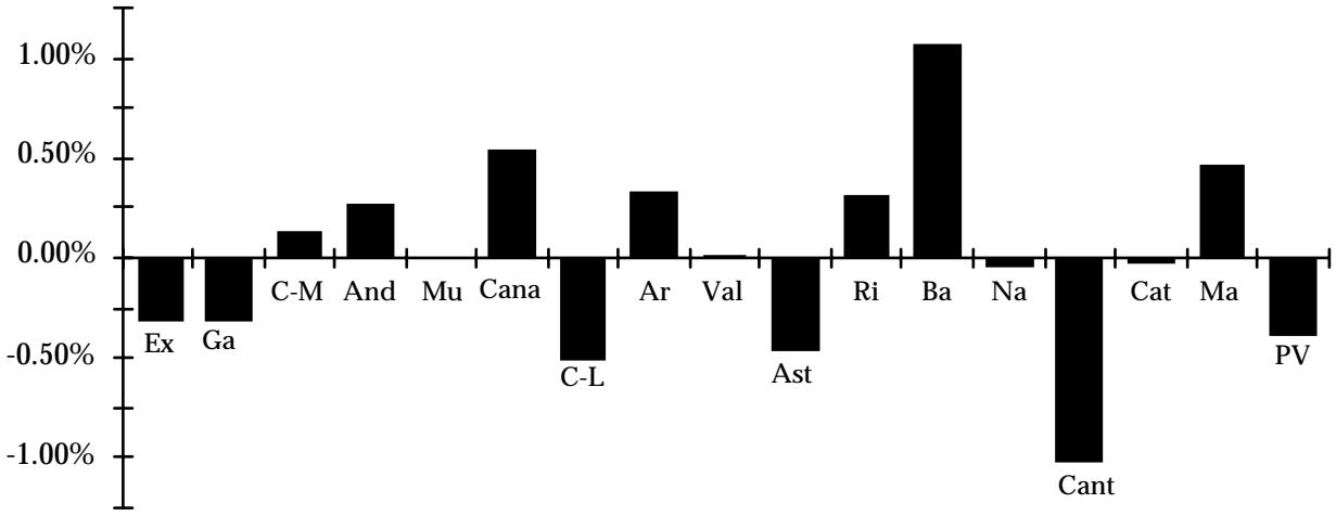
While the results are quite positive and in accordance with prior expectations, two unsatisfactory features of the model should be noted. The first one is that there remains an important error term which seems to have a systematic regional component. Figure 6 shows the average error for each region (averaging across subperiods), net of the prediction error corresponding to a hypothetical average region. A glance at this figure suggests that some of the largest errors have to do with sectoral considerations. The residual is positive and large (indicating better than expected performance) in Madrid and the island regions (with healthy, tourism-based economies), and negative and large in the (largely northern) regions which have suffered the most from the decline of basic manufacturing industries (such as steel-making and ship-building) and traditional small-scale agriculture.
Figure 6: Average residual of the growth equation without fixed effects
A second feature of the results which is not quite satisfactory is that the estimated model cannot generate convergence rates which are quite as high as the one we estimated in the previous section using a fixed-effects model (see Table 1).
It is easy to see that the rate of conditional convergence of output per worker (β) can be written as a weighted average of the rates of conditional convergence in TFP (ε) and in output per efficiency unit of labour (λ) where the weights are the fractions of the total deviation of relative productivity from its stationary value which are due to each of these two factors.8 Using the coefficients estimated in equation [6] and some additional information we can recover the rate of conditional convergence implied by the model and compare it with our benchmark estimate of 12.7%.
Since we have a direct estimate of ε, we only need to compute the rate of convergence of output per efficiency unit of labour towards its steady state in the average region. The average rate of depreciation implicit in the investment and capital stock series we are using is 0.043, the average rate of employment growth is -0.001, and the estimated average rate of technical progress at the midpoint of the sample period is given by
\[\mathrm{g} - \mathrm{c} ^ {*} 1 3. 5 = \frac {0 . 0 1 9 9}{0 . 6 4 8 2} - \frac {0 . 0 0 0 7 6}{0 . 6 4 8 2} 1 3. 5 = 0. 0 1 4 8 7.\]
8 If relative output per efficiency unit of labour, p, and relative technical efficiency, d, converge to their steadystate values at constant rates we will have
p =Ý λ(p - p )
and . Ý d = ε(d - d )
q = d + p )
The relative productivity of each region will then be given by q = p + d (with and we have
q =Ý ε(d - d ) + λ(p - p )
Under these assumptions q converges towards its steady state but, in general, not at a constant rate. We can, however, bound the rate of convergence of q in terms of ε and λ. Multiplying and dividing the right-hand side of the last expression by we have (q - q ) = (d - d )+ (p - p )
φ= ε d - d + λ p - p (q - ā), q - q q - q
which shows that the rate of convergence of q is a weighted average of ε and λ.
In a Solow-type model with human capital, the neoclassical convergence coefficient implied by these parameters would be given
\[(1 5) \lambda = (1 - \theta_ {\mathrm{k}} - \theta_ {\mathrm{h}}) (\delta + \mathrm{g} + \mathrm{n}) = (1 - 0. 3 5 1 8 - 0. 1 7 6 7) ^ {*} (0. 0 4 3 + 0. 0 1 4 8 7 - 0. 0 0 1) = 0. 0 2 6 8.\]
Using this figure and assuming, as a first approximation, that deviations of relative productivity from its steady-state value are due in equal parts to TFP and output per efficiency unit of labour, the estimated model implies a conditional convergence rate of productivity of
\[\beta = \frac {0 . 0 2 6 8 + 0 . 0 6 7 6}{2} = 0. 0 4 7 2,\]
which is considerably higher than the standard 2% but still much lower than our benchmark estimate.
A simple way to both of the problems we have just discussed is to reintroduce the regional dummies. Clearly, this is only a partial solution since the resulting fixed effects "hybrid" model, while able to empirically capture cross-regional TFP differences, will tell us nothing about what lies behind them. On the other hand, this specification does provide a useful way to gauge the extent to which regional disparities are due to factors not included in the model.
The significance of the dummies in our benchmark model suggests that countries or regions are very different from each other, but in what? According to our "structural" aggregate model, the answer would have to do with differences in the stocks and flows of physical, human and technological capital and the rate of employment growth. If this exhausted the list of relevant variables, the regional dummies should not be significant when we add them to equations like the ones we have just estimated. As we will presently see, this is not the case -- although the dummies do not "drive out" most of the variables we have considered either. This fact suggests that, while the factors identified by the theory have, in general terms, the expected effect, the models we have developed so far do not provide a completely satisfactory explanation of the immediate determinants of cross-regional differences in income levels and growth rates. It also remains to explain why certain regions accumulate factors faster than others, but this problem is probably best left to future research.
Table 4 shows the results of the estimation of equation (14) with and without the regional dummies after imposing constant returns to scale. Equation [6] is repeated from Table 3 to facilitate comparisons, equation [7] introduces fixed effects and equation [8] drops the relative level of education, which appears with a negative and insignificant coefficient in equation [7]. Finally, equation [9] is estimated after imposing the value of (the rate effect of human capital) obtained in equation [6]. Comparing the different columns of the table, we see that the coefficients of the production function and the average rate of technical progress are almost identical in all cases. The introduction of the fixed regional effects, however, has a dramatic effect on the estimated values of ε and and the treatment of the rate effect of human capital makes a noticeable difference in terms of the coefficients of the regional dummies.
9 See Mankiw, Romer and Weil (1992).
Table 4: Results with fixed regional effects
| [6] | (t) | [7] | (t) | [8] | (t) | [9] | (t) | |
| $\theta_k$ | 0.3518 | (6.18) | 0.3572 | (6.84) | 0.3411 | (6.56) | 0.332 | (6.30) |
| $\theta_l$ | [0.6482] | [0.6428] | [0.6589] | [0.668] | ||||
| $\theta_h$ | 0.1767 | (3.28) | 0.1823 | (3.52) | 0.1497 | (3.14) | 0.1297 | (2.69) |
| $\theta_u$ | 0.0301 | (0.23) | 0.0460 | (0.38) | 0.0539 | (0.44) | 0.0577 | (0.47() |
| $g\theta_l$ | 0.0199 | (3.20) | 0.0191232 | (2.25) | 0.0237 | (2.95) | 0,0265 | (3.26) |
| $c\theta_l$ | -0.00076 | (3.26) | -0.00075 | (3.42) | -0.0008 | (3.69) | -0.0008 | (3.79) |
| ε | 0.06765 | (3.63) | 0.2237 | (7.05) | 0.2166 | (6.90) | 0.2153 | (6.78) |
| μθl | 0.0201 | (2.44) | -0.0328 | (1.57) | [0.0201] | |||
| $R^2$ | 0.4629 | 0.5390 | 0.5331 | 0.5236 | ||||
| s.e. reg. | 0.02153 | 0.02036 | 0.0204 | 0.0206 | ||||
| θ|r_i: | ||||||||
| Madrid | 0.2973 | (4.60) | 0.2216 | (4.87) | 0.1729 | (3.69) | ||
| Baleares | 0.1579 | (4.28) | 0.1548 | (4.06) | 0.1525 | (3.94) | ||
| Cataluña | 0.1466 | (3.53) | 0.1164 | (3.00) | 0.0973 | (2.44) | ||
| País Vasco | 0.1132 | (2.59) | 0.0777 | (1.97) | 0.0551 | (1.36) | ||
| Navarra | 0.1042 | (2.40) | 0.0720 | (1.80) | 0.0514 | (1.26) | ||
| Rioja | 0.0617 | (1.67) | 0.0624 | (1.63) | 0.0633 | (1.63) | ||
| Valencia | [0.00] | [0.00] | [0.00] | |||||
| Aragón | 0.04822 | (1.31) | 0.0381 | (1.01) | 0.0315 | (0.82) | ||
| Canarias | 0.04332 | (1.13) | 0.0308 | (0.79) | 0.0226 | (0.57) | ||
| Asturias | -0.04711 | (1.31) | -0.0498 | (1.34) | -0.0513 | (1.36) | ||
| Andalucía | -0.07158 | (1.79) | -0.0538 | (1.36) | -0.0424 | (1.05) | ||
| Murcia | -0.06289 | (1.74) | -0.0593 | (1.58) | -0.0572 | (1.50) | ||
| Cast-León | -0.08696 | (2.39) | -0.0828 | (2.20) | -0.0799 | (2.09) | ||
| Cantabria | -0.07199 | (1.95) | -0.0841 | (2.24) | -0.0917 | (2.40) | ||
| Cast-Mancha | -0.1299 | (2.87) | -0.0910 | (2.31) | -0.0658 | (1.64) | ||
| Extremadura | -0.2444 | (5.00) | -0.2018 | (4.76) | -0.1742 | (4.02) | ||
| Galicia | -0.2681 | (5.16) | -0.2241 | (4.94) | -0.1954 | (4.22) | ||
| std. dev. θ|r_i: | 0.1153 | 0.0995 |
- Note: The coefficients shown inside brackets are imposed rather than estimated. In all cases we impose the assumption of constant returns to scale.
The speed of technological diffusion, measured by ε, increases dramatically, from 6.8 to 22% per year when regional dummies are added to the equation. This would seem to indicate that our previous estimate of this parameter suffered from a fixed-effects bias similar to the one which, according to Canova and Marcet (1995), biases towards zero estimates of the convergence rate obtained from unconditional growth regressions. To the extent that the TFP differentials across regions are due in part to non-transferable characteristics or are measured with error, the introduction of the dummies allows us to correct the problem, reducing the bias and increasing the estimated convergence coefficient. According to our estimates, the process of technological diffusion across regions is extraordinarily rapid and could very well generate (conditional) convergence in income levels at a rate over 12%. In fact, the unweighted average of the estimated ε and the value of λ implied by the model matches almost exactly our benchmark estimate of the rate of (conditional) convergence of productivity (see Table 5).
On the negative side, the loss of significance of the rate effect of human capital (measured by the coefficient µ, which is now negative) is rather discouraging. This result, however, may simply reflect the fact that there is relatively little temporal variation in the relative positions of the different regions in terms of educational attainment. Hence, the dummies may be picking up this effect along with other factors, such as the sectoral effects we have already discussed.10 Finally, the significance and size of the fixed effects suggest that much of the observed productivity differentials across regions are due to factors not captured by the model. After controlling for differences in factor endowments and for technological diffusion, there remain very significant cross-regional differences in steady-state productivity levels which the model captures but does not explain.
It may be of some interest to compare the estimates of the unexplained long-term productivity differentials generated by the different models in order to asses the extent to which the explicit consideration of factor accumulation and technological catch-up allows us to explain cross-regional differences. Table 5 summarizes the relevant information. The fixed-effects, non-structural model estimated in Section 3 gives us an "unrefined" or "gross" estimate of steady-state relative productivities which should in principle summarize all relevant differences across regions. This information is shown in column [2] of Table 5, which is taken from Table 1 (equation [2], after renormalizing the coefficients so that their average is exactly zero). Column [8] shows the steady-state productivity differentials implied by the coefficients of the regional dummies in the structural model with fixed effects. (This is equation [8] in Table 4, appropriately renormalized). Finally, column [9] shows the coefficients of the regional dummies obtained in equation [9] of Table 4 after imposing a positive rate effect from human capital (again, normalized so that their average is precisely zero). This last set of estimates may be interpreted as a refined "residual" and presumably summarizes the effects of a long list of factors which are not included in our aggregate model. Below the regional coefficients we show their standard deviation, a figure which we will interpret as a summary measure of the degree of unexplained long-term inequality. The last rows of the table summarize each model's predictions about the rate of conditional convergence of output (per worker and per efficiency unit of labour) and TFP levels for the case of an average region at the midpoint of the sample period.
Table 5: Unexplained long-run productivity differentials
R2
10 The of a regression of relative educational levels on regional dummies is 0.9198. Notice also that when we impose a positive value of µ in equation [9] the regional effects become noticeably smaller in many cases.
and implied convergence rates
| Equation = | [2] | [8] | [9] |
| "gross" relative productivities | =[2] net of factor acc. & catch up | =[8] net of rate effects of h. cap. | |
| Madrid | 29.79% | 22.59% | 17.94% |
| Baleares | 23.38% | 15.91% | 15.90% |
| Cataluña | 19.24% | 12.07% | 10.38% |
| País Vasco | 16.95% | 8.20% | 6.16% |
| Navarra | 10.50% | 7.63% | 5.79% |
| Rioja | 2.83% | 6.67% | 6.98% |
| Aragón | 4.94% | 4.24% | 3.80% |
| Canarias | 3.37% | 3.51% | 2.91% |
| Valencia | 3.38% | 0.43% | 0.65% |
| Asturias | -4.10% | -4.55% | -4.48% |
| Andalucía | -9.44% | -4.95% | -3.59% |
| Murcia | -7.72% | -5.50% | -5.07% |
| Cast. y León | -10.73% | -7.85% | -7.34% |
| Cantabria | 2.04% | -7.98% | -8.52% |
| Cast. la Mancha | -15.60% | -8.67% | -5.93% |
| Extremadura | -28.40% | -19.75% | -16.77% |
| Galicia | -40.42% | -21.98% | -18.89% |
| std. deviation | 17.53% | 11.53% | 9.95% |
| implied rates of conditional convergence: | |||
| output per worker (β) | 0.1273 | 0.1240 | 0.1253 |
| output per eff. unit (λ) | 0.0314 | 0.0353 | |
| technical efficiency (ε) | 0.2166 | 0.2153 | |
- Note: The rates of conditional convergence of output per efficiency unit are calculated using the same procedure as outlined above in the text. The figure given in the table for the rate of convergence of productivity is the unweighted average of ε and λ.
Comparison of columns [2] and [8] shows that the estimates of productivity differentials generated by the structural and non-structural models are very similar in terms of the regional ranking they induce. Although both sets of estimates are of the same order of magnitude, those obtained using the structural model are significantly smaller. In particular, controlling for factor accumulation and technological catch-up reduces the unexplained level of income dispersion by about one third (the standard deviation drops from 17.53% to 11.53%). To the extent that the regional fixed effects may also be capturing the rate effects from human capital, this second figure may overstate somewhat the amount of unexplained inequality. Column [9], where we impose what may be a reasonable guess as to the size of such effects, provides a lower bound on the extent of unexplained disparities, with a standard deviation of 9.95%. The reduction of the standard deviation which results from the introduction of the new human capital variable is quite small, essentially because, given the high estimated rate of convergence, the effect of human capital differentials on steady-state relative productivities is also small.
In conclusion, accounting for factor stocks and flows and for technological diffusion reduces the unexplained long-term dispersion of productivity levels by somewhere between one third and one half. This still leaves us with a lot of unexplained variation in steady-state relative productivities or, to put it differently, with the conclusion that there is still a lot of work to do before we can say with any degree of confidence that we understand satisfactorily the determinants of regional productivity.
6.- The sources of convergence
In a series of papers Danny Quah (1993, 1995a, b and c) has criticized the use of growth regressions on the grounds that the estimated coefficients, while providing a convenient way to summarize the behaviour of a "typical" country or region, cannot tell us anything about intradistribution dynamics which is the key issue at hand. To get around this limitation, Quah proposes abandoning growth regressions in favour of the estimation of, ideally, the stochastic kernel which governs the evolution of the whole distribution and, in practice, a matrix of transition probabilities across segments of a discretized distribution. Being somewhat unfair, one could say that these techniques give us little more than pretty pictures of a moving distribution, but no information on what is driving the motion.11
Although Quah's criticism is sound as far as it goes, there is no reason why the analysis should stop with the inspection of the estimated coefficients. In this section I will try to show that the results of a growth equation can be used to generate a good deal of information about the immediate sources of changes in the distribution of income -- and lots of pretty pictures as well. The "convergence accounting" exercise we will undertake provides, in particular, a rough decomposition of observed income convergence into a number of components which reflect the impact of technological diffusion and the accumulation of various types of factors. This is, admittedly, only half (and the easiest half of) the problem, for it does tell us very little about the ultimate causes of differences in growth patterns. But it is a start, and it may give us some clues as to where to look for deeper answers.
The exercise we propose is simply to use the estimated model (in particular, equation [8] in Table 4) and the underlying data to decompose observed productivity growth rates. After imposing the assumption of constant returns to scale and omitting the (non-significant) rate effects from human capital, equation (14) can be written in the form
\[(1 6) \Delta \mathbf {y} _ {\mathrm{it}} - \Delta \mathbf {l} _ {\mathrm{it}} = \theta_ {\mathrm{l}} (\mathbf {g} + \varepsilon \widetilde {\mathbf {r}} _ {\mathrm{v}}) + \theta_ {\mathrm{l}} c t + \theta_ {\mathrm{k}} (\Delta \mathbf {k} _ {\mathrm{it}} - \Delta \mathbf {l} _ {\mathrm{it}}) + \theta_ {\mathrm{h}} \Delta h _ {\mathrm{it}} + \theta_ {\mathrm{u}} \Delta u _ {\mathrm{it}}\]
11 Being fair, these techniques are a nice complement of other types of analysis but remain purely descriptive devices. They can be quite useful in identifying interesting patterns and regularities (such as the emergence of the polarized, twin-peaked distribution identified by Quah in various samples) but, by their very nature, cannot give us any information about the forces shaping the process, even at a modest "growth accounting" level.
\[- \varepsilon \biggl (\widetilde {\mathbf {y}} _ {\mathrm{it}} - \theta_ {\mathrm{k}} \widetilde {\mathbf {k}} _ {\mathrm{it}} - \theta_ {\mathrm{l}} \widetilde {\mathbf {l}} _ {\mathrm{it}} - \theta_ {\mathrm{h}} \widetilde {\mathbf {h}} _ {\mathrm{it}} - \theta_ {\mathrm{u}} \widetilde {\mathbf {u}} _ {\mathrm{it}} - \sum_ {\mathrm{i} \neq \mathrm{v}} \Gamma_ {\mathrm{i}} D R E G _ {\mathrm{i}} \biggr) + \omega_ {\mathrm{it}},\]
with the rate of productivity growth in the left-hand side. Since we are focusing on convergence it will be convenient to work with productivity growth differentials relative to a hypothetical average region rather than with "gross" growth rates. Treating such a hypothetical region (endowed with average productivity growth, average (log) factor stocks and growth rates and average TFP) as another observation, we can write
\[(1 7) \Delta \mathbf {y} _ {\mathbf {t}} - \Delta \mathbf {l} _ {\mathbf {t}} = \theta_ {\mathbf {l}} (\mathbf {g} + \varepsilon \widetilde {\mathbf {r}} _ {\mathbf {v}}) + \theta_ {\mathbf {l}} c t + \theta_ {\mathbf {k}} (\Delta \mathbf {k} _ {\mathbf {t}} - \Delta \mathbf {l} _ {\mathbf {t}}) + \theta_ {\mathbf {h}} \Delta \mathbf {h} _ {\mathbf {t}} + \theta_ {\mathbf {u}} \Delta \mathbf {u} _ {\mathbf {t}} + \varepsilon \Gamma + \omega_ {\mathbf {t}}\]
where Γ is the average value of for i v and the "prediction error" for the average region (i.e. the difference between the observed average growth rate of productivity and the model's prediction for the average region). Subtracting the second equation from the first, we can write the growth rate of relative productivity in region i, , as a weighted sum of (log) factor stocks and factor accumulation rates, all measured in deviations from the contemporaneous sample average:
\[\begin{array}{l} \text {(18)} \Delta \mathrm {q_ {it}} = \theta_ {\mathrm{k}} (\widetilde {\Delta k} _ {\mathrm{it}} - \Delta \widetilde {l} _ {\mathrm{it}}) + \theta_ {\mathrm{h}} \Delta \widetilde {h} _ {\mathrm{it}} + \theta_ {\mathrm{u}} \Delta \widetilde {u} _ {\mathrm{it}} \\ \quad - \varepsilon \left(\widetilde {y} _ {\mathrm{it}} - \theta_ {\mathrm{k}} \widetilde {k} _ {\mathrm{it}} - \theta_ {\mathrm{l}} \widetilde {l} _ {\mathrm{it}} - \theta_ {\mathrm{h}} \widetilde {h} _ {\mathrm{it}} - \theta_ {\mathrm{u}} \widetilde {u} _ {\mathrm{it}} + \Gamma - \sum_ {\mathrm{i} \neq \mathrm{v}} \Gamma_ {\mathrm{i}} D R E G _ {\mathrm{i}}\right) + \omega_ {\mathrm{it}} - \omega_ {\mathrm{t}}. \end{array}\]
Lumping the (very small) cyclical component of relative growth, ∆u together with the error term, we can express the growth rate of relative productivity as the sum of a residual and three components which measure the contribution of capital deepening human capital investment and technological diffusion to the relative growth performance of each region. The capital deepening component, may be further disaggregated into the separate contributions of gross capital formation and employment growth:
\[\mathrm{G} _ {\mathrm{qz}} = \mathrm{G} _ {\mathrm{qk}} + \mathrm{G} _ {\mathrm{ql}} + \theta_ {\mathrm{k}} \widetilde {\Delta \mathrm{k}} _ {\mathrm{it}} + (- \theta_ {\mathrm{k}} \widetilde {\Delta \mathrm{l}} _ {\mathrm{it}}). \tag {19}\]
Table 6 summarizes the results of the growth decomposition. For each region we show the average value (across subperiods) of relative productivity growth and each of its components, together with the initial value of relative productivity. Using this information we can now undertake two simple exercises which will allow us to quantify the contribution of each of these components to observed (unconditional) convergence in output per employed worker. First, we will regress each of the components of growth on initial relative productivity. The slope coefficient of each of these partial convergence regressions will give us the rate of (unconditional) beta convergence which would have been observed in a hypothetical world in which the relative productivity of each region changed due only to each factor at a time, with all regions displaying average behaviour in all other categories. Secondly, we will compute the relative productivity of each region at the end of the sample period under the same assumption and calculate the standard deviation of the resulting counterfactual distribution. Comparing this figure with the observed value of the same inequality indicator at the beginning of the period, we will have an estimate of the degree of sigma convergence induced by each of the components. Because one has to worry about the covariance terms, neither of our partial (beta and sigma) convergence measures necessarily adds up to observed total convergence. Taken together, however, these two exercises should give us a rough idea of "how much" of observed convergence can be traced to the behaviour of factor stocks and technological diffusion.
Table 6: Sources of relative productivity growth
| q64 | $G_q$ | $G_{ql}$ | $G_{qk}$ | $G_{qh}$ | $G_{qa}$ | residual | |
| Extremadura | -44.71% | 0.75% | 0.04% | 0.32% | 0.18% | 0.19% | 0.01% |
| Galicia | -44.04% | 0.48% | 0.13% | 0.01% | 0.12% | 0.22% | -0.01% |
| Cast. Mancha | -27.28% | 0.49% | 0.27% | 0.00% | 0.26% | -0.04% | 0.00% |
| Andalucía | -22.88% | 0.44% | 0.06% | 0.01% | 0.09% | 0.27% | 0.02% |
| Murcia | -13.15% | 0.12% | -0.24% | 0.09% | -0.05% | 0.31% | 0.00% |
| Canarias | -11.80% | 0.78% | -0.33% | 0.53% | -0.05% | 0.63% | 0.02% |
| Cast. y León | -10.72% | -0.06% | 0.32% | -0.18% | 0.00% | -0.20% | 0.00% |
| Aragón | 0.10% | 0.18% | 0.14% | -0.22% | -0.01% | 0.28% | -0.01% |
| Valencia | 0.24% | 0.09% | -0.21% | 0.36% | 0.01% | -0.07% | 0.00% |
| Asturias | 1.74% | -0.48% | 0.21% | -0.44% | 0.00% | -0.26% | 0.00% |
| Rioja | 9.65% | -0.09% | 0.10% | 0.24% | -0.06% | -0.38% | -0.01% |
| Baleares | 15.09% | 0.58% | -0.23% | 0.67% | 0.00% | 0.15% | -0.01% |
| Navarra | 17.20% | -0.25% | -0.06% | -0.15% | -0.01% | -0.02% | -0.01% |
| Cantabria | 18.88% | -0.70% | 0.17% | -0.46% | -0.02% | -0.40% | 0.00% |
| Cataluña | 34.21% | -0.75% | -0.26% | 0.05% | -0.06% | -0.48% | -0.01% |
| Madrid | 38.71% | -0.47% | -0.44% | 0.04% | -0.35% | 0.29% | -0.01% |
| País Vasco | 38.77% | -1.12% | -0.08% | -0.50% | -0.06% | -0.49% | 0.01% |
- Notes: q is relative productivity, the observed growth rate of relative productivity (calculated as the average over all subperiods of the observed productivity growth differential relative to the hypothetical average region). is the growth differential induced by "component" x of productivity growth, with l = employment growth, k = physical capital accumulation, human capital accumulation, a = technological diffusion. The "residual" is the sum of the "cyclical perturbation" proportional to the change in the unemployment rate and the prediction error relative to the average region. Components of relative productivity growth are computed using the estimated model with fixed regional effects, equation [8] in Table 4.
The results are presented in Table 7. The first three columns of the table show the initial and (observed or counterfactual) final values of the standard deviation of relative productivity and the percentage reduction of this indicator of regional inequality during the sample period. The remaining columns show the slope coefficients and summary statistics of a set of (unconditional) regressions of relative productivity growth and each of its components on initial relative productivity. Figures 7 to 12 show the corresponding scatters and the fitted regression lines.
Let us focus first on the three-way decomposition of convergence in terms of educational investment, capital deepening and technological diffusion. Each of these three components would induce, by itself, a significant amount of both beta and sigma convergence. In both cases, the sum of the three components roughly adds up to total convergence, and their contributions are of the same order of magnitude, with education contributing between 20 and 25% of the total, technological diffusion accounting for roughly a third of observed convergence, and the evolution of the capital/labour ratio taking up the remaining 40% or so. The decomposition of this last factor into the separate contributions of capital accumulation and employment growth, finally, shows that progress towards the equalization of capital/labour ratios has come more from the reallocation of employment across regions than from capital flows (or higher domestic investment) in the poorer regions. This finding is consistent with the view that the large migratory flows of the sixties and early seventies contributed substantially to regional convergence in Spain.12 In recent years, moreover, continuing convergence in productivity levels may have come, to some extent, at the expense of an increase in regional unemployment disparities.
Table 7: Immediate sources of convergence in output per employed worker
| std. dev. of relative productivity | unconditional convergence reg. | |||||
| 1964 | 1991 | %Δ | beta | (t) | R2 | |
| observed values: | 0.2518 | 0.1558 | -38.14% | 1.72% | (5.07) | 0.6314 |
| counterfactuals, growth due only to change in: | ||||||
| physical capital | 0.2518 | 0.2438 | -3.18% | 0.34% | (1.06) | 0.0694 |
| employment | 0.2518 | 0.2318 | -7.94% | 0.39% | (1.90) | 0.1938 |
| human capital | 0.2518 | 0.2276 | -9.63% | 0.37% | (4.46) | 0.5704 |
| technological catch up | 0.2518 | 0.2230 | -11.46% | 0.61% | (2.16) | 0.2377 |
| capital/labour ratio | 0.2518 | 0.2109 | -16.24% | 0.73% | (3.24) | 0.4116 |
12 See for example Raymond and García (1996).
Figure 7: Observed beta convergence in relative productivity
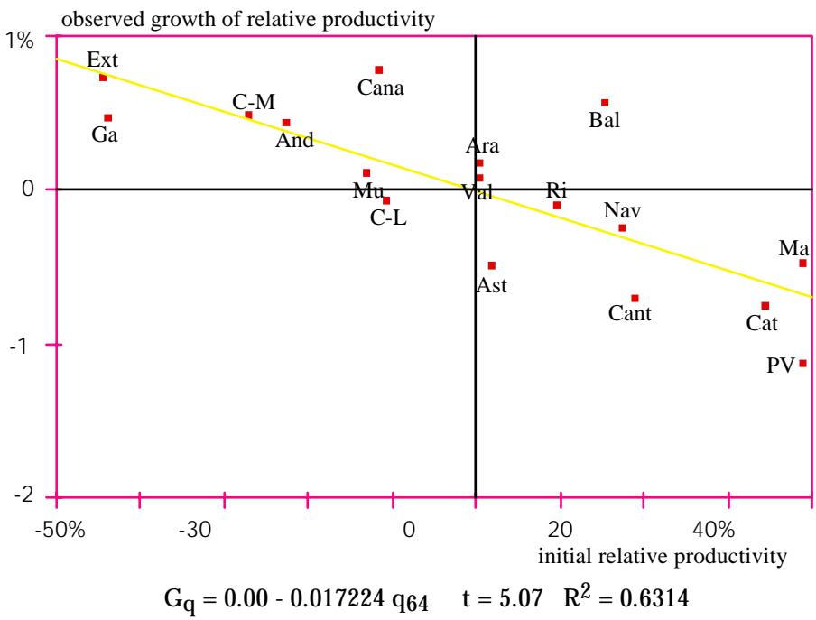
Figure 8: Beta convergence in productivity induced by the evolution of the capital/labour ratio
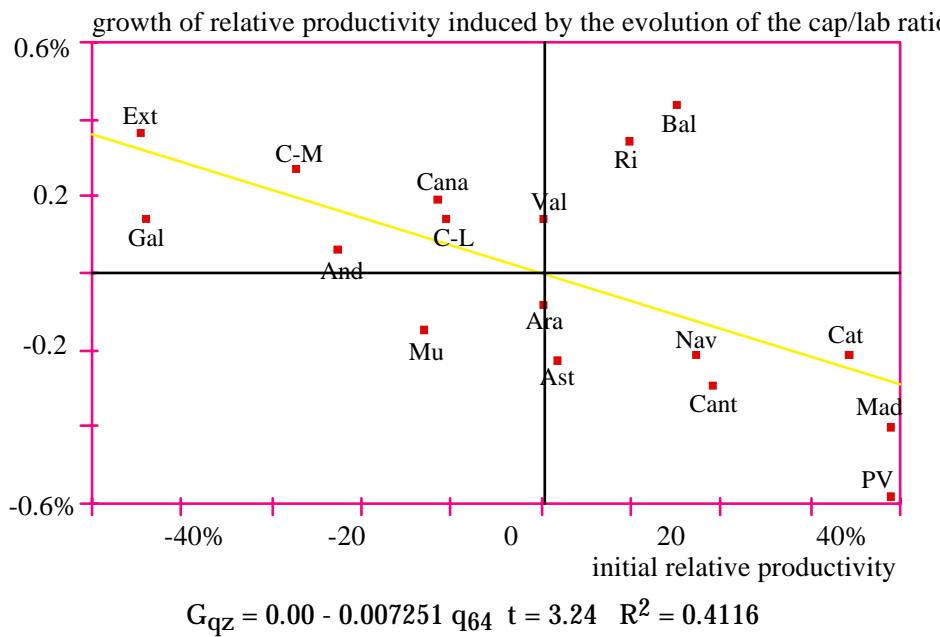
Figure 9: Beta convergence in productivity induced by (gross) physical capital accumulation
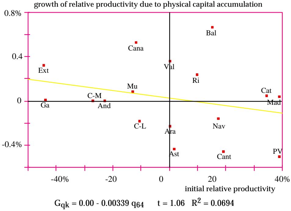
Figure 10: Beta convergence in productivity induced by employment growth
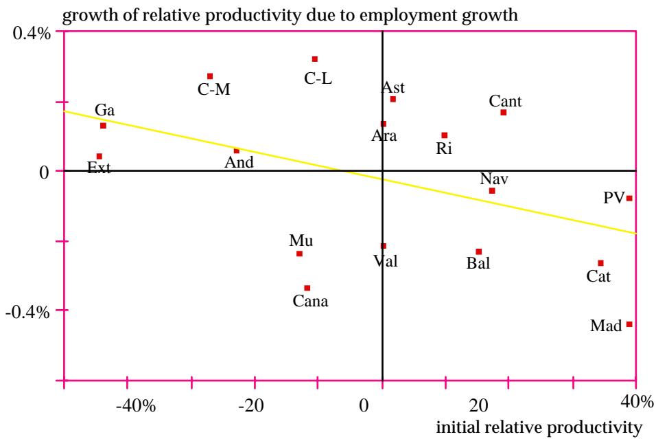
\[\mathrm {G_ {ql} = 0.00- 0.003861^ {*} q_ {64} \quad t = 1.90 R^ {2} = 0.19377}\]
Figure 11: Beta convergence in productivity induced by human capital accumulation
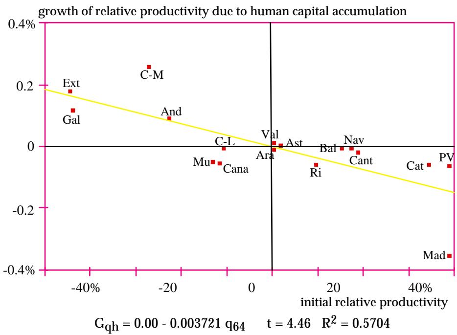
Figure 12: Beta convergence in productivity induced by technological diffusion
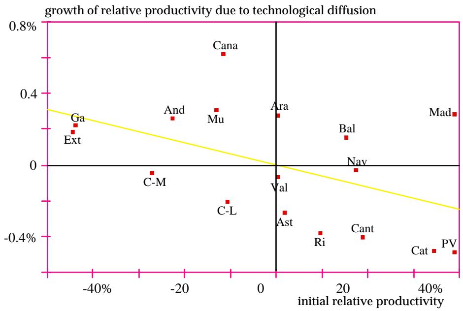
\[\mathrm {G_ {qa} = 0.00- 0.006147^ {*} q_ {64} \quad t = 2.16\quad R^ {2} = 0.23767}\]
7.- The role of sectoral structure
One variable which is usually significant in regional convergence regressions is (some indicator of) the sectoral composition of output or employment. One possible interpretation of this result is that the inclusion of such variables helps control for sectoral shocks. There may be, however, a lot more than this to the story. First of all, the reallocation of resources across sectors -- and particularly the decrease in the weight of agriculture in the poorest regions -- may be an important source of convergence. In the first part of this section I will supply some evidence that this is indeed the case. Secondly, I will observe that there are important differences across sectors in convergence patterns. This suggests that working with disaggregated data may be a good strategy to improve our understanding of the operation of convergence mechanisms and the determinants of regional incomes in the medium and long run.
a.- Sectoral structure and convergence
It is well known in the regional economics literature that productivity differences across regions have an important sectoral component. To the extent that average productivities vary significantly across sectors, differences in the sectoral composition of employment can generate important productivity disparities across regions. Figure 13 suggests that this effect may be important since productivity differences across sectors are marked and persistent, particularly in the case of agriculture.
Figure 13: Evolution of relative sectoral productivities - Note: Logarithm of output per job in each sector (average over all regions), measured in deviations from average (across regions) log output per job in the same year.
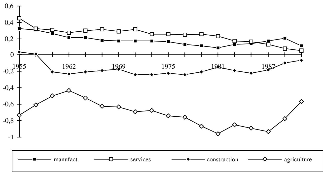
From a dynamic perspective, the homogeneization of sectoral structures could explain a considerable part of the observed reduction in regional income disparities in Spain. Figures 13 and 14 suggest, in particular, that the evolution of agricultural employment may have played a crucial role in the process. At the beginning of the sample period (1955-91), farming absorved a very important fraction of total employment, particularly in the poorest regions. Although the negative correlation between the weight of agriculture and average regional productivity has not changed, the flow of labour out of agriculture and into other sectors with higher productivities has been more intense in the poorer regions, thus contributing to bring their income levels closer to the national average.
To quantify the contribution of this process to convergence, I will borrow an idea from Marimón and Zilibotti (1996) and construct what they call a virtual economy. Although this sounds terribly sophisticated, the idea is very simple: we just calculate the path of relative output per worker in each region under different counterfactual assumptions about the sectoral composition of employment and the behaviour of sectoral productivities in each region. Then, we will apply the usual apparatus of convergence regressions and σ plots to the resulting fictional economies and compare the results with those corresponding to the observed path of the relevant variables. The experiment will allow us to isolate the contribution of sectoral change to regional convergence.
Figure 14: Relative regional productivity vs. weight of agriculture in total employment, 1955 - Note: Both the weight of agriculture in total employment (shareagric) and productivity (measured by the log of regional output per job, q) are measured in deviations from the regional average. The fitted regressionline is given by
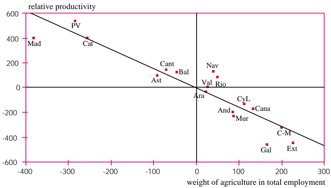
\[\mathrm{q} = - 1. 5 5 3 \text { shareagric } \quad \mathrm{t} = 9. 7 7 \quad \mathrm{R} ^ {2} = 0. 8 6 4.\]
If we repeat the exercise with 1991 data, the slope coefficient is very similar and the fit is even better 0.932). The weight of the agricultural sector, however, is now much lower in all regions. The decline is much more marked in the regions where the initial weight of agriculture was highest.
We will construct, in particular, two virtual economies. The first one respects the observed path of average sectoral productivities in each region but assumes that the sectoral composition of employment has not changed since 1955. By construction, any convergence we observe in this artificial economy must be due to the convergence of productivities -- both across sectors and across regions within the same sector. The second virtual economy is constructed under the opposite assumption: we now respect the observed sectoral shares in employment for each of the regions but assume that average sectoral productivities remain constant over time at their initial values. Income convergence will now be due exclusively to the homogeneization of the sectoral structures of the different regions. Although observed convergence is not, strictly speking, the sum of the convergences we would observe in each of these counterfactual economies, the exercise should give us some idea of the relative importance of the two sources of convergence we have identified.13
13 Our data allows a disaggrgation of regional output and employment into four sectors (agriculture, manufacturing, services and construction) since 1955. Since employment at the sectoral level is measured by the number of jobs (which differs from the number of employed workers), we work with this measure of productivity also at the aggregate regional level. Hence, our data differ from the one used in previous sections both in the sample period, which is now longer since we do not use data on factor stocks, and in the measure of productivity.
Table 8: Convergence in productivity: observed pattern and two counterfactual scenarios
| - | unconditional converg. | |||||
| cv. of log output per job | ||||||
| eq. | 1955 | 1991 | %Δ | β | (t) | R2 |
| observed values | 0.2798 | 0.1027 | -63.31% | 0.0186 | (16.2) | 0.946 |
| counterfactual scenarios: | ||||||
| 1955 employment structure | 0.2798 | 0.1749 | -37.49% | 0.0119 | (6.58) | 0.743 |
| 1955 sectoral productivities | 0.2798 | 0.1861 | -33.50% | 0.0111 | (5.38) | 0.659 |
Table 8 summarizes the results. The first three columns show the initial and final values of an index of the dispersion of regional productivities (the coefficient of variation of log output per job) in each of the scenarios (the observed one and the two countefactuals) and the percentage change in this measure of inequality. The last three columns summarize the results of the corresponding unconditional convergence regressions in relative productivities. Figures 15 and 16 show in greater detail the patterns of sigma and beta convergence in each of the scenarios.
Figure 15: σ-convergence in output per job, 1955-91 observed pattern and two counterfactual scenarios
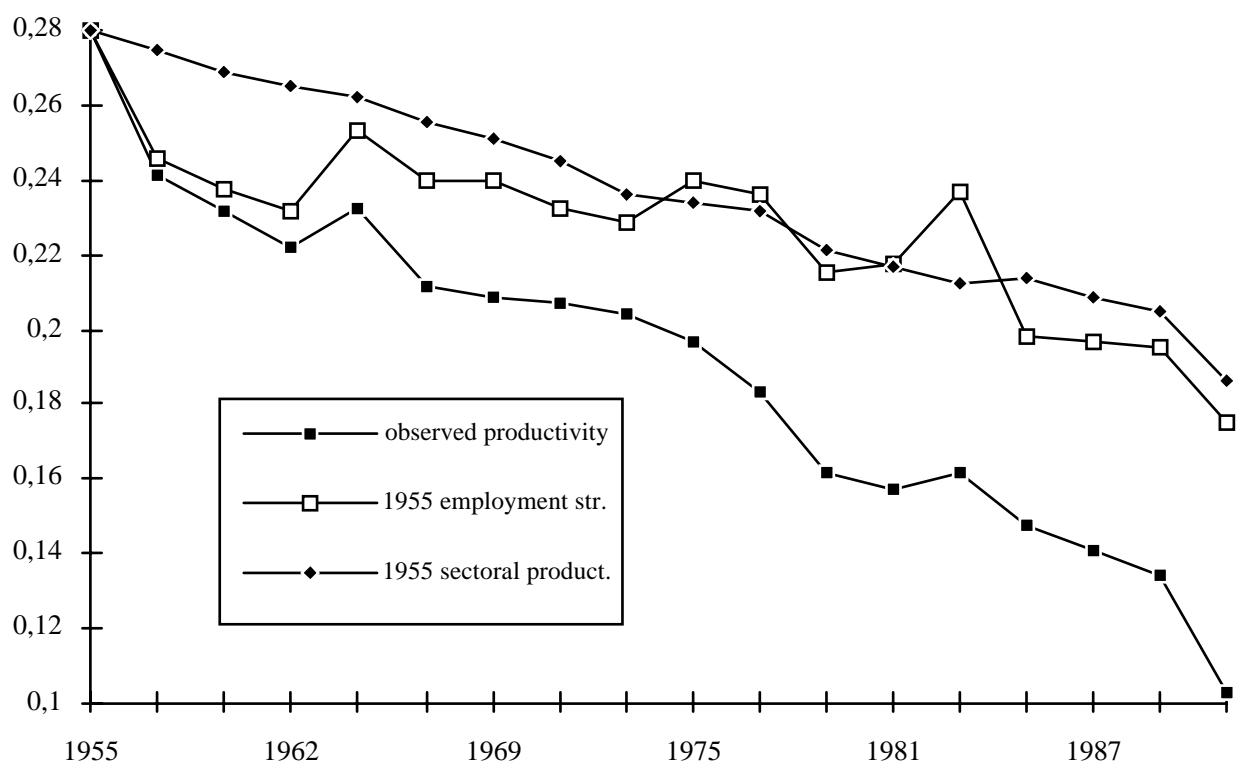
- Note: the figure shows the standard deviation of relative productivity in each scenario.
Figure 16: β−Convergence in output per job, 1955-91 a.- observed values
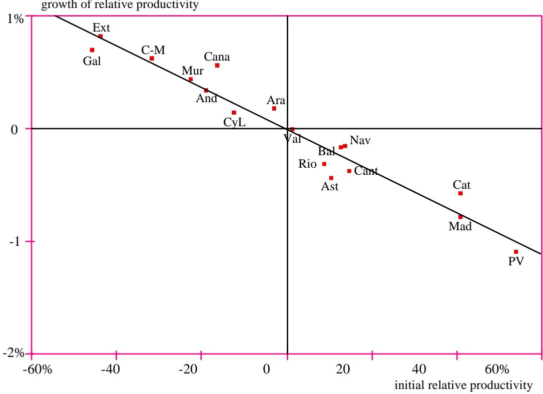
b.- constant sectoral weights in total employment (1955 values) c.- Constant sectoral productivities (1955 values)
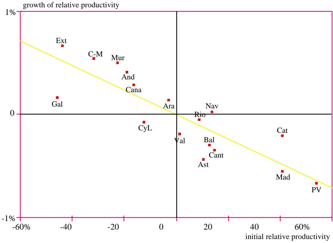
growth of relative productivity - Notes: the output variable is relative productivity, defined as the logarithm of real output per job measured in differences with the sample average of the same variable in each period. The dependent variable is the growth rate of relative productivity over the period 1955-91, and the independent variable is relative productivity in 1955. The different panels of the figure show the fitted regression line in each of the scenarios.
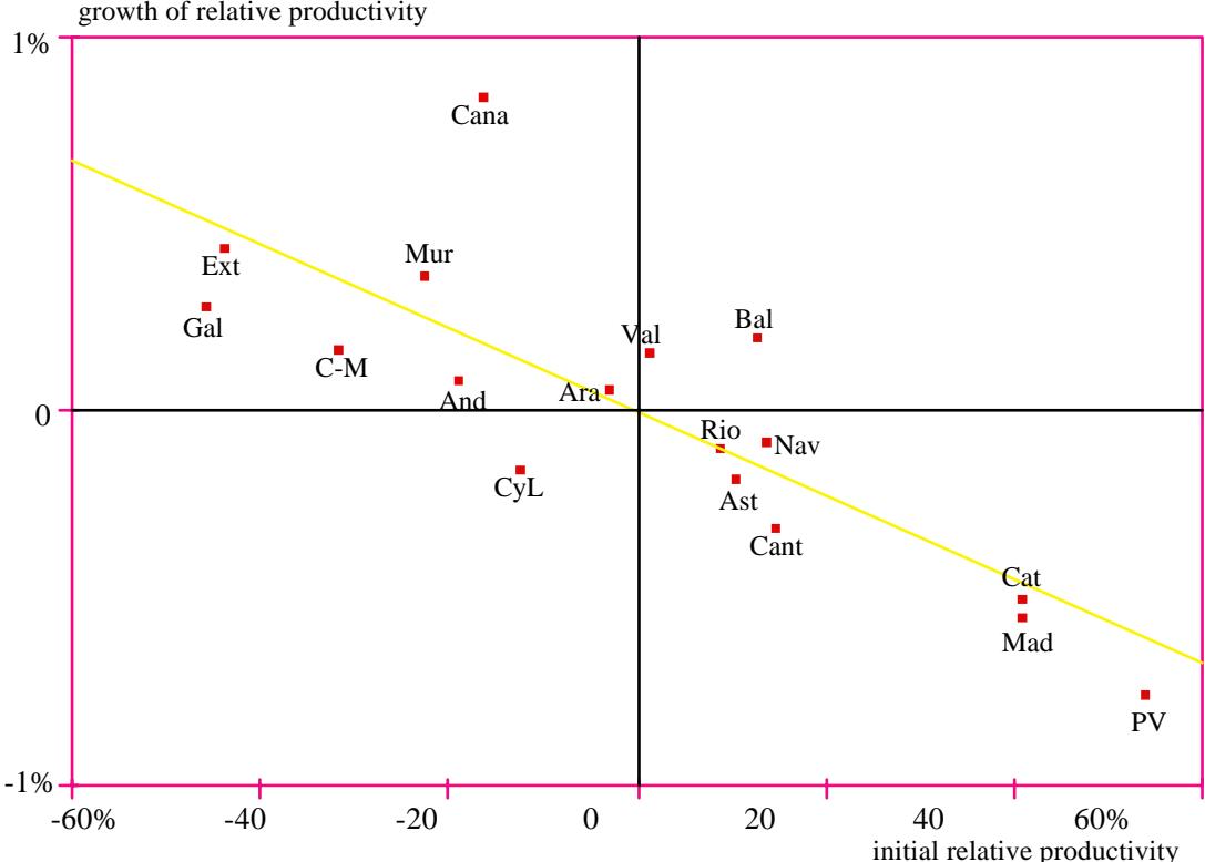
The results suggest that both the evolution of the sectoral structure and the behaviour of productivity have contributed significantly to regional convergence. We observe, first, that each of these factors induces a significant amount of convergence in average regional productivities. Both hypothetical beta convergence coefficients are significantly different from zero and the dispersion of regional productivities falls by about one third in each of the virtual economies. Secondly, the two effects are approximately of the same magnitude, both in terms of the estimated value of β and of the reduction in σ each of them would induce by itself. It seems fair to conclude, therefore, that approximately one half of the observed convergence is due to sectoral factors.
b.- Sectoral convergence patterns
One of the "lessons" of the previous exercise is that aggregates hide many things. When we disaggregate we often run into interesting questions which suggest new lines of research. If we can answer these questions at least partially, we will gain a better understanding of the mechanisms which govern the evolution of the regional income distribution and, possibly, a greater ability to influence them.
Table 9: β-convergence in output per job
| unconditional regression | regional agg. | manufacturer. | services | construction | agriculture | |||||
| coef | (t) | coef | (t) | coef | (t) | coef | (t) | coef | (t) | |
| β | 0.0347 | (5.29) | 0.0825 | (6.43) | 0.0428 | (4.06) | 0.1952 | (7.71) | 0.0586 | (3.86) |
| sectoral y* | 0.0000 | 0.1171 | (4.05) | -0.0191 | (0.26) | -0.1792 | (11.1) | -0.6325 | (7.12) | |
| $R^2$ | 0.1128 | 0.1373 | 0.0569 | 0.2182 | 0.0527 | |||||
| s.e. | 0.0190 | 0.0364 | 0.0245 | 0.0478 | 0.0830 | |||||
| conditional regression | ||||||||||
| β | 0.1252 | (6.04) | 0.1313 | (7.38) | 0.0892 | (5.28) | 0.2539 | (8.22) | 0.1800 | (6.70) |
| Andalucía | -0.0930 | (2.39) | -0.0248 | (0.36) | -0.0748 | (1.02) | -0.0355 | (0.67) | 0.0108 | (0.09) |
| Aragón | 0.0486 | (1.25) | 0.0507 | (0.72) | 0.0124 | (0.17) | 0.0509 | (0.97) | 0.1355 | (1.14) |
| Asturias | -0.0081 | (0.21) | 0.2332 | (3.34) | -0.0217 | (0.28) | -0.1191 | (2.26) | -0.6179 | (5.16) |
| Baleares | 0.0958 | (2.46) | -0.2052 | (2.90) | 0.0916 | (1.20) | 0.0320 | (0.61) | -0.0756 | (0.64) |
| Canarias | 0.0263 | (0.66) | 0.0622 | (0.89) | -0.0182 | (0.24) | 0.0553 | (1.05) | -0.0533 | (0.45) |
| Cantabria | 0.0208 | (0.53) | 0.1046 | (1.47) | 0.0653 | (0.90) | -0.0449 | (0.85) | -0.2107 | (1.77) |
| Cataluña | 0.1844 | (4.60) | 0.0484 | (0.69) | 0.1240 | (1.64) | 0.0269 | (0.51) | 0.2350 | (1.98) |
| Cast. la Mancha | -0.1243 | (3.12) | -0.0761 | (1.09) | -0.1382 | (1.91) | -0.0579 | (1.10) | 0.1470 | (1.23) |
| Castilla y León | -0.0960 | (2.46) | 0.0981 | (1.41) | -0.0867 | (1.19) | -0.0295 | (0.56) | -0.0729 | (0.61) |
| Extremadura | -0.2490 | (6.18) | 0.0430 | (0.58) | -0.2120 | (2.81) | -0.0987 | (1.88) | -0.1678 | (1.41) |
| Galicia | -0.3396 | (8.49) | -0.0067 | (0.10) | -0.0945 | (1.30) | -0.1132 | (2.15) | -0.6535 | (5.49) |
| Madrid | 0.2617 | (6.64) | 0.0936 | (1.34) | 0.1705 | (2.27) | 0.0504 | (0.96) | 0.0355 | (0.30) |
| Murcia | -0.0532 | (1.36) | -0.0972 | (1.38) | -0.0783 | (1.04) | 0.0632 | (1.20) | 0.0714 | (0.60) |
| Navarra | 0.0909 | (2.34) | -0.0439 | (0.62) | 0.0561 | (0.78) | 0.0485 | (0.92) | 0.4167 | (3.50) |
| País Vasco | 0.2022 | (4.89) | 0.1326 | (1.86) | 0.1032 | (1.37) | 0.0151 | (0.29) | 0.3195 | (2.69) |
| Rioja | -0.0002 | (0.01) | -0.2590 | (3.56) | 0.0580 | (0.80) | 0.0810 | (1.54) | 0.4168 | (3.50) |
| Valencia | 0.0327 | (0.84) | -0.1536 | (2.17) | 0.0433 | (0.58) | 0.0754 | (1.43) | 0.0633 | (0.53) |
| $R^2$ | 0.1975 | 0.2468 | 0.1100 | 0.2749 | 0.1800 | |||||
| s.e. | 0.0186 | 0.0350 | 0.0245 | 0.0474 | 0.0795 | |||||
| average $y_i^*$ | 0.0000 | 0.1407 | 0.1191 | -0.1784 | -0.6904 | |||||
| std. dev. of $y_i^*$ | 0.1493 | 0.1243 | 0.0998 | 0.0655 | 0.2921 | |||||
- Note: All variables measured in logs and expressed in deviations from the interregional average of (log) output per job in the same period. The one exception are the estimated regional steady states within each sector (the coefficients of the regional dummies), which are measured in deviations from the inter-regional average for
the corresponding sector. The t statistic shown next to each of these coefficients is the one appropiate for testing the hypothesis that, in terms of the relevant sector, each region is not different from the average. The specification is the same one we used in Table 1.
One of the first things that one sees when working with disaggregated data is that convergence patterns and the regional distribution of (estimated) long-term relative productivity levels are quite different across sectors. To illustrate this fact I will repeat two already familiar exercises, imitating once more the work of other authors.14 Figure 17 shows the pattern of sigma convergence at the aggregate and sectoral levels. While the regional dispersion of agricultural productivity increases over time, the value of σ in the construction and service sectors displays marked oscillations without a clear trend. Only the manufacturing sector displays a sustained reduction in the dispersion of regional productivities. Table 9 reveals a somewhat more uniform pattern of beta convergence. The estimated convergence rate is always positive but varies, in a specification with regional dummies, between 8.9% in the service sector and 25.4% in construction. Estimates of long-term relative productivities also vary significantly across sectors for many regions.
Investigating the sources of these differences may give us a more complete picture of the determinants of regional income and its evolution than the one we can get from an aggregate model. As a framework for this type of analysis we will need to develop models which allow us to analyze jointly the evolution of productivity and sectoral structure. These models should allow a more detailed and micro-oriented analysis of the different convergence mechanisms and the determinants of long-term regional incomes. They shoul allow us to deal explicitly with factors such as regional comparative advantage, based on endowments of fixed factors or in cumulative experience in certain sectors, and to explore the possible importance of various types of inter- or intra-sectoral externalities.15 Policy implications could be important. If sectoral structure matters and comparative advantage in high value added sectors is something which can be acquired with experience, for example, an interventionist industrial policy could be justified, at least from the point of view of each region, since the sectoral composition of investment could be as important as its aggregate volume.
8.- Summary and conclusions
A host of papers have found a negative partial correlation between output per capita (or per worker) and subsequent growth. The strength of this correlation, which is often taken as a measure of the speed of convergence, varies considerably across papers reflecting differences in specification.
14 See Raymond and García (1994) and García-Milà and Marimón (1995). Barro and Sala (1991) also run convergence regressions at the sectoral level with US data. Although they find some differences across sectors in the estimated convergence rates, these are smaller than in the Spanish case and these authors prefer to emphsize the overall stability of the convergence pattern rather than worry about the sources of sectoral differences.
15 Some of these issues are beginning to attract the attention of researchers. See for example García-Milà and McGuire (1992 and 1993), Carlino and Voith (1992), Marimón and Zilibotti (1996) and Goicolea, Herce and Lucio (1995).
Estimates of the rate of convergence obtained with unconditional convergence equations (at the regional level), or controlling for investment rates in physical and human capital (at the national level) are typically quite low and cluster around a central value of 2% per year. Recently, however, a number of authors have obtained much higher estimates of the speed of convergence using more flexible specifications which allow more room for regional or national specificities.
From a theoretical perspective these recent estimates are somewhat problematic. Slow convergence can be given a sensible interpretation within a standard neoclassical model as an indication that the technology displays close to constant returns to scale in a broad capital aggregate which includes cumulative investment in education. Within the same framework, however, very fast convergence either takes us back to the old-fashioned neoclassical model with a narrow interpretation of capital (implying that investment in intangibles is not productive), or cannot be explained at all. In this paper we have argued that these results must be taken as an indication that the standard model used in the literature does not take into account some important convergence mechanisms such as technological diffusion and sectoral reallocation.
The bulk of the article investigates, using data for the Spanish regions, the extent to which it is possible to explain observed convergence patterns and cross-regional productivity differentials in terms of an extension of the aggregate neoclassical model which allows for technological diffusion and rate effects from human capital. Our starting point is a non-structural convergence model with fixed regional effects à la Canova and Marcet (1995). While this specification is essentially a black box, it does allow us to estimate the distribution of regional productivities to which the sample may be expected to converge in the long run provided "things remain equal", and the speed of convergence of the regional economies towards their stationary relative productivity levels. As in Canova and Marcet (1995) and other related papers, the results indicate that this stationary distribution is characterized by a high level of inequality (slightly above the observed level), and that convergence towards it is very fast .
We use the results of this non-structural, dummy-variable model as a benchmark to evaluate the performance of an aggregate structural model which extends the standard neoclassical model by partially endogenizing the rate of technical progress. We proceed essentially by asking to what extent the introduction of the variables suggested by standard growth theory allows us to fit the data (i.e. to generate convergence rates and sustained productivity differentials comparable to those estimated using the benchmark model) without resorting to the use of regional dummies.
The results of the exercise are mixed. On the positive side, our structural model yields very reasonable estimates of the parameters of the production function and we find evidence of a rapid process of technological diffusion across regions. These findings suggest that a suitably extended aggregate model may provide an adequate framework for a first approximation to the analysis of growth and convergence. On the other hand, a version of the model without fixed regional effects presents large and systematic regional residuals which point to important omitted variables and predicts convergence rates which are much lower than our benchmark estimate.
Both problems can be "fixed" through the introduction of fixed regional effects to capture productivity differentials due to unobserved regional characteristics. This gives us a "hybrid" model which generates conditional convergence at just about the right speed and reproduces almost perfectly the observed pattern of relative productivity growth. This model is used to quantify the contribution to the reduction of regional inequality of technological diffusion (around one third) and factor accumulation (two thirds, including human capital), and to provide an estimate of the amount of long-term inequality which is not explained by either of these factors (around one half in the best of cases).
One obvious limitation of the "hybrid model" is that, while it allows us to empirically capture and quantify the effects of unobserved regional characteristics, it gives us no information about their nature. Some of our results, however, seem to indicate that sectoral factors may be responsible for at least part of the unexplained productivity differentials and point towards a more disaggregated analysis as a promising strategy for future research. The last part of the paper provides some preliminary evidence which is consistent with this hypothesis.
- References
- Banco Bilbao-Vizcaya (antes Banco de Bilbao). Renta nacional de España y su distribución provincial.. Banco Bilbao-Vizcaya, varios años.
- Banco de Bilbao. Renta nacional de España y su distribución provincial. Serie homogénea 1955-75. Banco de Bilbao, 1977.
- Barro, R. and X. Sala i Martin. "Economic Growth and Convergence Across the United States." NBER Working Paper no. 3419, Aug. 1990.
- Barro, R. and X. Sala i Martin. "Convergence across States and Regions." Brookings Papers on Economic Activity 1, 1991, pp. 107-82.
- Barro, R. and X. Sala i Martin. "Convergence." Journal of Political Economy, 100(2), 1992a, pp. 223-51.
- Barro, R. and X. Sala i Martin. "Regional Growth and Migration: A Japan-United States Comparison." Journal of the Japanese and International Economies 6, 1992b, pp. 312-46.
- Baumol, W. "Productivity Growth, Convergence and Welfare: What the Long-Run Data Show." American Economic Review 76(5), Dec. 1986, pp. 1072-85.
- Canova, F. and A. Marcet. "The Poor Stay Poor: Non-convergence across Countries and Regions." CEPR Discussion Paper no. 1265, 1995.
- Carlino, G. and R. Voith. "Accounting for Differences in Aggregate State Productivity." Regional Science and Urban Economics, 22, 1992, pp. 597-617.
- Coulombe, S. and F. Lee (1993). "Regional Economic Disparities in Canada." Mimeo, University of Ottawa.
- de la Fuente, A. "Catch-up, Growth and Convergence in the OECD." CEPR Discussion Paper no. 1274, 1995.
- de la Fuente, A. "The empirics of growth and convergence: a selective review." Journal of Economic Dynamics and Control 21(1), Jan. 1997, pp. 23-74.
- Dolado, J., J. M. González-Páramo and J. M. Roldán. "Convergencia Económica entre las Provincias Españolas: Evidencia Empírica (1955-1989)." Moneda y Crédito 198, 1994, pp. 81-131.
- Dowrick, S. and D. T. Nguyen. "OECD Comparative Economic Growth 1950-85: Catch-up and Convergence." American Economic Review 79(5), Dec. 1989, pp. 1010-1030.
- Fundación BBV. El stock de capital en la economía española. Bilbao, 1995.
- Garcia-Milá, T. and T. McGuire. "Growth, Industrial Mix and Structural Change in US Regions: the Shift to a Service-based Economy." Mimeo, 1993.
- Garcia-Milá, T. and T. McGuire. "Industrial Mix as a Factor in the Growth and Variability of States Economies." Mimeo, 1992.
- García Milá, T. and R. Marimón. "Integración regional e inversión pública en España," in R. Marimón (editor), La economía española en una Europa diversa. Junio de 1995 (forthcoming by Antoni Bosch).
- Goicolea, A., J. A. Herce and J. J. de Lucio. "Patrones territoriales de crecimiento industrial en España." Documento de trabajo 95-14, FEDEA, 1995.
- Islam, N. "Growth Empirics: A Panel Data Approach" Quarterly Journal of Economics CX(4), 1995, pp. 1127-70.
- Mankiw, G. "The Growth of Nations." Brookings Papers on Economic Activity I, 1995, pp. 275-326.
- Mankiw, G., D. Romer and D. Weil. "A Contribution to the Empirics of Economic Growth." Quartely Journal of Economics CVII(2) 1992, pp. 407-37.
- Marcet, A. "Los pobres siguen siendo pobres: Convergencia entre regiones y países, un análisis bayesiano de datos de panel," en Crecimiento y convergencia regional en España y Europa, Vol. II. Instituto de Análisis Económico, Barcelona, 1994.
- Marimón, R. and F. Zilibotti. "Actual vs. virtual employment in Europe: Is Spain different?" CEPR Discussion Paper no. 1427, 1996.
- Mas, M., J. Maudos, F. Pérez and E. Uriel. "Disparidades regionales y convergencia en las comunidades autónomas." Revista de Economía Aplicada, 4, 1994, pp. 129-48.
- Mas, M., F. Pérez, E. Uriel and L. Serrano.Capital humano, series históricas 1964-92; Fundación Bancaja, Valencia, 1995.
- Quah, D. "Galton's Fallacy and Tests of the Convergence Hypothesis." CEPR Discussion Paper no. 820, July 1993.
- Quah, D. "Convergence empirics across economies with (some) capital mobility." Center for Economic Performance, Discussion Paper no. 257, 1995a.
- Quah, D. "Empirics for economic growth and convergence." CEPR Discussion Paper no. 1140, 1995b.
- Quah, D. "Twin Peaks: Growth and convergence in models of distribution dynamics." Mimeo, LSE, 1995c.
- Raymond, J. L. and B. García. "Las disparidades en el PIB per cápita entre comunidades autónomas y la hipótesis de convergencia." Papeles de Economía Española 59, 1994, pp. 37-58.
- Raymond, J. L. and B. García. "Distribución regional de la renta y movimientos migratorios." Papeles de Economía Española 67, 1996, pp. 185-201.
- Romer, P. "Crazy Explanations for the Productivity Slowdown."NBER Macroeconomics Annual 2,1987, pp. 163-210.
- Sala i Martin, X. On Growth and States. Tesis doctoral no publicada, Harvard University, 1990.
- Sala i Martin, X. "The Classical Approach to Convergence Analysis." CEPR Discussion Paper no. 1254, Oct. 1995.
- Sala, X. "Regional Cohesion: Evidence and Theories of Regional Growth and Convergence." European Economic Review 40, 1996, pp. 1325-52.
Shioji, E. "Regional Growth in Japan." Mimeo, Yale University, 1992.
Figure 17: σ-convergence in sectoral productivities, 1955-91
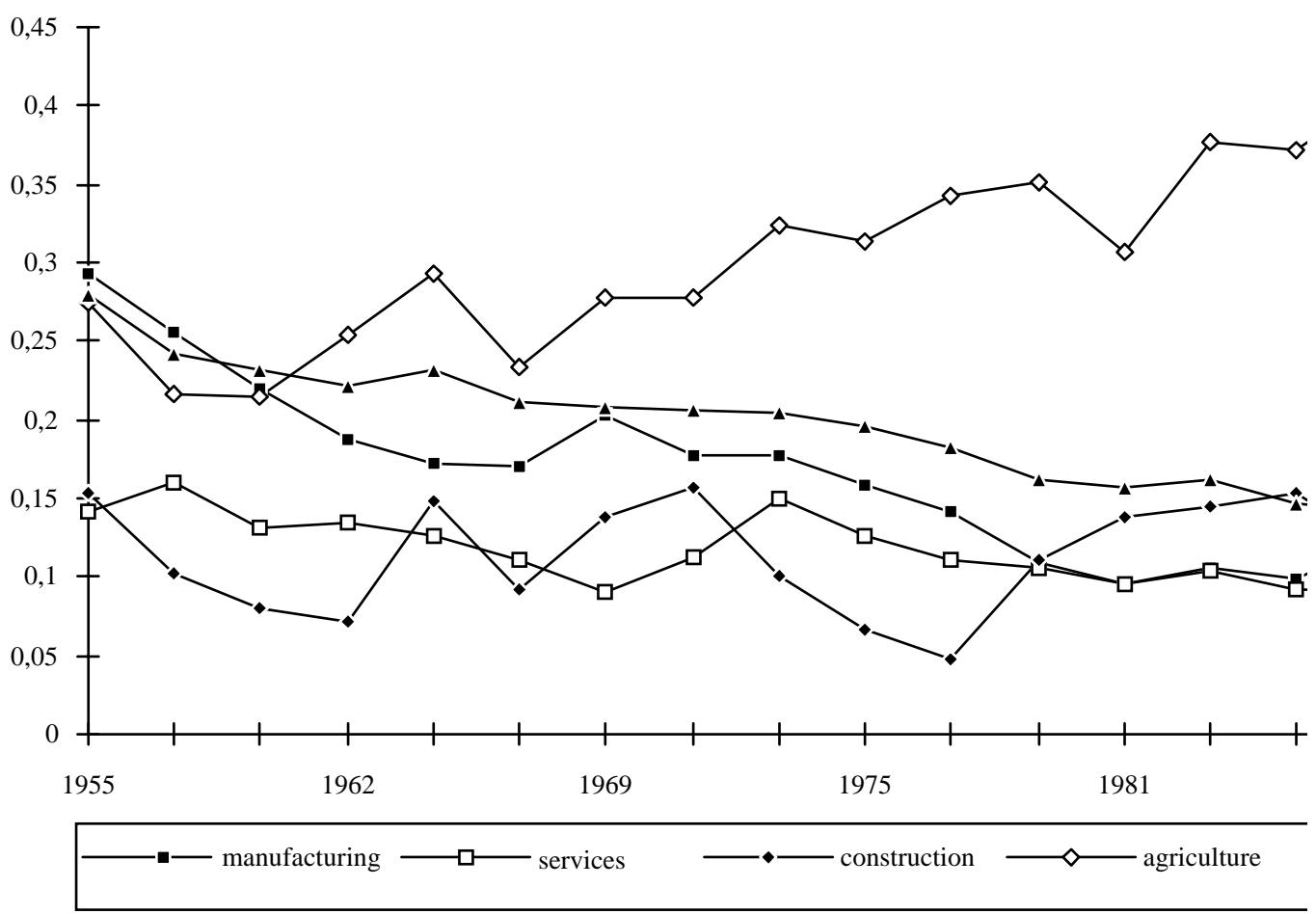
Este texto se ha extraído automáticamente del documento original. Para citarlo o leerlo con su maquetación, descargue el PDF.
Descargar en PDF