II Jornada sobre el sistema público de pensiones y seguridad social
Delayed-Retirement Incentives in Spain: Evaluating Lump-Sum Commutation and Actuarial Fairness
AHMED ACIÓN LÓPEZ
CARLOS VIDAL-MELIÁ
Estudios sobre la Economía Española 2026/25 Septiembre 2026
fedea
Las opiniones recogidas en este documento son las de sus autores y no coinciden necesariamente con las de Fedea.
* Este trabajo forma parte de un proyecto de investigación financiado parcialmente por la Fundación Ramón Areces
Ahmed Ación López
Department of Economics and Law, University of Cassino and Southern Lazio, Cassino, Italy. (e-mail: ahmed.acionlopez@unicas.it). ORCID: 0000-0001-9211-0909.
Carlos Vidal-Meliá (corresponding author)
Department of Financial Economics and Actuarial Science and Instituto Universitario de Derecho Patrimonial – Patrimonium, University of Valencia, Valencia, Spain. (email: carlos.vidal@uv.es). ORCID: 0000-0002-7227-5076.
Abstract
Spain’s delayed-retirement rules allow eligible workers to choose between a permanent pension supplement, a statutory lump sum, or a mixed option. This paper evaluates whether exchanging the life-contingent supplement for the lump sum is actuarially neutral and examines how behavioral and institutional channels affect the financial comparison. The analysis combines income-stratified mortality, a simulation grid of 280 institutionaldemographic profiles, and population weights derived from the 2024 Continuous Sample of Working Lives (MCVL). Under dynamic segmented mortality, the baseline MCVLweighted ratio of the lump sum to the actuarial present value of the foregone supplement is 0.512, and none of the simulated profiles reaches actuarial neutrality. The shortfall is larger for women and higher-pension profiles because the lump-sum formula is concave in pension entitlement and does not incorporate longevity differences. Tax treatment, policy risk, and present-oriented discounting can make commutation financially defensible for some profiles. In the most favorable combined scenario, profiles reaching financial indifference represent 39.38% of the MCVL-weighted population and contain 8.0 percentage points of the observed 24.02% lump-or-mixed take-up rate. Under the central CRRA specification, the MCVL-weighted certainty-equivalent gap is 3.0%, although this welfare result is conditional on the maintained assumptions. The findings support clearer actuarial information and a review of the statutory formula, while distinguishing formula non-neutrality from the rationality of individual choices.
JEL Classification: H55; D14; D91; G22; J26
Keywords: actuarial neutrality; delayed retirement; longevity risk; lump-sum commutation; pension design.
Acknowledgments
We are grateful to Juan Manuel Pérez-Salamero and Anna Castañer-Garriga for generously providing the initial datasets from the Continuous Sample of Working Lives (MCVL).
Declarations
Conflict of Interest: The authors have no competing interests to declare that are relevant to the content of this article.
Funding: Carlos Vidal-Meliá gratefully acknowledges financial support from the Generalitat Valenciana, Spain, through the PROMETEO 2025 programme for research excellence groups (project CIPROM/2024/075).
Code and Input Data Availability Statement: The paper is based on a reproducible R implementation of a scenario-based actuarial model for delayed retirement in Spain. The analysis combines external mortality inputs with a computational framework that generates the full set of statutory, actuarial, fiscal, welfare, and behavioral outputs used in the paper. The full R code and input files are available from the authors upon request and will be deposited in a public repository with a citable DOI upon acceptance, to support transparency and reproducibility.
Declaration of generative AI and AI-assisted technologies in the writing process: During the preparation of this work, the authors used ChatGPT (OpenAI) and Abacus.AI (ChatLLM Teams) to assist with language editing and to check and debug the R code underlying the analysis. These tools were not used to design the analysis, generate results, or produce any of the reported findings. All modelling choices, computations, results, and interpretations were carried out, reviewed, and validated by the authors, who take full responsibility for the content of the manuscript.
Delayed-Retirement Incentives in Spain: Evaluating Lump-Sum Commutation and Actuarial Fairness.
1. Introduction
The sustainability of public pay-as-you-go pension systems has become a central policy concern across advanced economies, driven by population ageing, rising life expectancy, the retirement of large post-war cohorts, and slower GDP growth. In Spain, these pressures have shaped the pension reform agenda over the past decade and led to successive legislative changes aimed at improving financial sustainability while preserving benefit adequacy (Conde-Ruiz & González, 2016; Vegas Sánchez et al., 2013). The reform trajectory has shifted markedly between the 2013 and 2023 legislative packages. The 2013 reform relied on automatic adjustment mechanisms, notably the Sustainability Factor and the Pension Revaluation Index (IRP), which strengthened longrun solvency but at the cost of reducing the real value of pensions (Díaz-Giménez & Díaz-Saavedra, 2017). Their subsequent suspension and repeal altered the direction of reform and renewed concerns about intertemporal solvency and intergenerational distribution (Díaz-Giménez & Díaz-Saavedra, 2026). This diagnosis is reinforced by recent actuarialbalance-sheet assessments, which document substantial long-term solvency pressures in the Spanish public pension system (Garvey et al., 2023; Castañer et al., 2025).
Rather than relying on automatic benefit adjustments, recent Spanish pension reforms have increasingly emphasized delayed retirement as a mechanism for improving financial sustainability. Postponing retirement increases contribution revenues while shortening the expected benefit-payment period. An actuarial assessment of these incentives requires comparing the compensation offered with the value of the pension rights affected by later claiming (Jiménez & Viola, 2023). Law 21/2021 increased the existing permanent pension supplement and added a statutory lump-sum alternative. Subsequent regulatory development introduced the mixed option and specified the implementation of the three alternatives. Although this arrangement increases flexibility, the lump-sum formula does not explicitly incorporate survival prospects and is not calibrated directly to the actuarial value of the foregone pension supplement.
This issue is not merely theoretical. Evidence from the 2023 and 2024 editions of the Continuous Sample of Working Lives (Muestra Continua de Vidas Laborales, MCVL) shows that 17.90% of delayed retirees chose the pure lump-sum option in 2023 and 21.36% in 2024; when the mixed option is included, the corresponding shares rise to 18.48% and 24.02%, respectively (Dirección General de Ordenación de la Seguridad Social, 2024, 2025). If the commuted amount is not actuarially equivalent to the foregone annuity increment, individuals may relinquish longevity insurance in return for compensation that departs materially from its underlying pension value.
From a comparative perspective, Spain’s institutional design is distinctive because it offers immediate capital as a statutory alternative to the lifelong delayed-retirement supplement. Although lump-sum mechanisms have existed in a limited number of countries, permanent pension increases remain the predominant form of delayedretirement incentive across advanced public pension systems (Department for Work and Pensions, 2026; Australian Government, 2026; Spasova et al., 2025). The Spanish arrangement therefore provides a particularly relevant setting for examining the actuarial terms of commutation.
The primary objective of this paper is to evaluate whether the Spanish statutory commutation formula provides an actuarially neutral exchange for the foregone lifecontingent pension supplement. The paper does not estimate a structural model of retirement or payout choice. Instead, it separates the valuation of the statutory exchange from the individual circumstances that may make immediate capital attractive.
Relative to recent Spanish studies of individual choice, observed reform responses, and budgetary effects (Contreras, 2024; Devesa et al., 2024; de la Fuente, 2023), this paper places the statutory commutation formula itself at the centre of the analysis. Its specific contribution is to evaluate that formula across heterogeneous pension and mortality profiles and to map the resulting actuarial diagnostics onto the observed delayedretirement population using MCVL weights. Behavioral, institutional, and welfare analyses are used as interpretive extensions.
The analysis proceeds in three layers. The primary layer compares the statutory lump sum with the actuarial present value of the foregone supplement and reports breakeven horizons, internal rates of return, and death-before-breakeven probabilities. The second introduces heterogeneous discounting, subjective survival beliefs, taxation, and policy risk to assess when the financial ranking may change. The third provides an exploratory certainty-equivalent analysis under CRRA and Stone–Geary preferences. This hierarchy preserves the distinction between actuarial non-neutrality, individual financial attractiveness, and welfare.
Under the baseline dynamic segmented specification, the statutory lump sum represents, on average, 51.2% of the actuarial present value of the foregone pension supplement once the simulations are weighted using the 2024 MCVL population distribution. Consistent with this result, none of the 280 simulated profiles reaches actuarial neutrality. In the most favorable combined behavioral and institutional scenario, profiles reaching financial indifference represent 39.38% of the MCVL-weighted population. These profiles account for 8.0 percentage points of the observed 24.02% lump-or-mixed take-up rate. Under the central CRRA calibration, population weighting reduces the mean relative certaintyequivalent gap from 5.86% to 3.00%. These results qualify the interpretation of individual choices without altering the finding that the statutory formula is not actuarially neutral.
After this introduction, Section 2 reviews the related literature on delayed-retirement incentives, behavioral explanations for annuity avoidance, and actuarial neutrality. Section 3 presents the institutional setting, data sources, representative profiles, their mapping to MCVL cells, and the methodological framework. Section 4 reports the main actuarial results and derives population-relevant magnitudes using MCVL weights. Section 5 examines behavioral, fiscal, and policy-risk extensions, including their combined effect. Section 6 provides an exploratory welfare evaluation based on certaintyequivalent measures under maintained assumptions. Section 7 discusses the interpretation and policy implications of the findings, distinguishing actuarial non-neutrality from individual welfare conclusions. Section 8 concludes. The Appendix briefly describes the supplementary workbook and Supplementary Data File S1, which provide the numerical outputs and MCVL population weights underlying the main text.
2. Literature Review: Delayed Claiming, Lump-Sum Preferences, and Actuarial Neutrality
Population ageing has led many pension systems to introduce delayed-retirement credits intended to encourage later claiming and longer working lives. In contributory pension schemes, these adjustments are commonly assessed against an actuarial-neutrality benchmark, but statutory rates vary across countries and do not necessarily preserve pension wealth at the individual level (Queisser & Whitehouse, 2006; OECD, 2025). Their value depends on mortality, discount rates, pension entitlement, and claiming age, so the financial attractiveness of delay may differ substantially across individuals and groups (Orszag, 2001; Knoll & Olsen, 2014; Mitchell & Maurer, 2018).
A related literature examines why many individuals claim public pension benefits at relatively early ages and whether alternative payout forms can alter this decision. In the United States, early claiming remains common even though delay increases monthly benefits and may raise lifetime benefits for some claimants (Knoll & Olsen, 2014). Evidence from the United Kingdom and the United States further indicates that more generous adjustments for delayed claiming can affect claiming behavior, although responses vary across demographic groups and institutional settings (Gorry et al., 2023; Slavov, 2025).
2.1. The Annuity Puzzle and the Preference for Liquidity
The choice between a life-contingent pension increment and an immediate lump sum is closely related to the annuity puzzle. Under restrictive assumptions, including the absence of bequest motives and sufficiently complete markets, life annuities protect individuals against longevity risk and can support higher lifetime welfare (Davidoff et al., 2005; Yaari, 1965). These results do not imply, however, that complete annuitization is optimal for every retiree.
Empirical evidence confirms that payout choices are sensitive to institutional and household circumstances. In the United Kingdom, purchases of conventional annuities fell sharply after the introduction of the Pension Freedoms, while drawdown arrangements became more common (Cannon et al., 2016). Evidence from Switzerland also shows substantial heterogeneity in the choice between annuities and lump sums (Bütler & Teppa, 2007). Bequest motives, psychological ownership and the desire to retain control over accumulated wealth can increase the attraction of immediate capital, while tax treatment may also materially influence payout choices (Lockwood, 2012; Shu & Shu, 2018; Bütler & Ramsden, 2024). Experimental evidence also cautions against assuming that lump-sum recipients necessarily consume the payment too rapidly, as retirees may instead preserve or even oversave a substantial part of the capital received (Fatás et al., 2013).
How the alternatives are presented also matters. Brown et al. (2008) show that lifetime annuities are substantially more attractive when framed in consumption terms than when described as investments. Beshears et al. (2014) likewise find that the appeal of annuitization changes when its insurance value and consumption consequences are made more salient. Extending this evidence to a European pension setting, Bockweg et al. (2018) find that consumption, investment, gain, and loss frames affect the allocation between lifetime income and a partial lump sum. Brown et al. (2016), in turn, show that alternative descriptions of Social Security claiming consequences affect expected claiming ages. Together, these findings indicate that observed choices may depend not only on underlying financial values but also on how lifetime income, immediate capital, gains from delay, and losses from early claiming are presented.
2.2. Behavioral Mechanisms and Retirement Decisions
Present-biased preferences and time inconsistency provide one explanation for the attraction of immediate payments. Individuals who place disproportionate weight on current consumption may value immediate capital more strongly than an equivalent stream of future pension income (Laibson, 1997; Schreiber & Weber, 2016). Evidence of substantial heterogeneity in discounting among older individuals further suggests that retirement and saving decisions cannot be adequately represented by a single common discount rate (Huffman et al., 2019).
The form in which delayed-retirement compensation is paid may influence claiming and retirement behavior independently of its actuarial value. Experimental and simulation studies indicate that actuarially adjusted lump-sum incentives can encourage later benefit claiming and, in some settings, later retirement relative to equivalent annuity increments (Fatás et al., 2007; Chai et al., 2013; Maurer et al., 2018, 2021; Maurer & Mitchell, 2021; Bachmann et al., 2023). These findings establish that payout form affects behavior, but they do not by themselves determine which option produces greater individual welfare.
Subjective survival expectations constitute another relevant mechanism. O’Dea and Sturrock (2023) find that pessimistic survival beliefs can explain a substantial part of observed non-annuitization, whereas Jeong et al. (2025) conclude that belief errors generate under-annuitization but account for only a limited share of the broader annuity puzzle. Information interventions can also produce different effects depending on their content: education about claiming rules and longevity may improve pension outcomes, while some framing interventions may delay claiming without necessarily improving financial welfare (Glenzer et al., 2025). Decision aids that make longevity risk and lifetime pension income more transparent may therefore improve the quality of retirement choices without presuming that one payout form is universally preferable (Rose & Morrison, 2018).
2.3. Actuarial Neutrality and Statutory Commutation
Actuarial fairness and actuarial neutrality are related but distinct concepts. Actuarial fairness concerns the relationship between lifetime contributions and benefits, whereas actuarial neutrality is generally a marginal benchmark for assessing whether accrued pension wealth changes with retirement timing (Queisser & Whitehouse, 2006). The present paper applies the same present-value logic to payout form. A commuted lump sum is actuarially neutral when it equals the present value of the life-contingent pension income surrendered by the claimant, under a specified mortality table and discount rate. This benchmark is useful for evaluating pension design, but it is not a normative requirement and does not imply that an actuarially equivalent payment maximizes welfare for every individual. Liquidity constraints, health, bequests, taxation, risk preferences, and other household resources may justify choosing either option even when their actuarial values differ.
Previous proposals for lump-sum delayed-retirement credits have generally sought to preserve approximate actuarial equivalence while changing the timing and salience of compensation (Orszag, 2001; Chai et al., 2013; Mitchell & Maurer, 2018). The distinction between payout form and actuarial value is therefore important. A lump sum may encourage delayed claiming because it is more salient or liquid, while a separate question is whether the amount paid adequately reflects the value of the annuity increment that has been commuted.
The Spanish literature has begun to examine the incentives created by the recent delayedretirement reform. Jiménez and Viola (2023) place these measures within the broader demographic and financial challenges facing the pension system. Contreras (2024) evaluates the lump-sum option by calculating the survival period required for the annuity increment to exceed the immediate payment and examines how this threshold varies with pension entitlement, contribution history, discounting and sex. Devesa et al. (2024) analyse early administrative evidence on responses to the reform and its pensionexpenditure implications, while de la Fuente (2023) focuses on its budgetary effects.
Together, these studies provide institutional, empirical and fiscal perspectives, but they do not systematically evaluate the actuarial value of the statutory commutation formula across heterogeneous pension and mortality profiles.
3. Data and methodology
3.1. Data, Institutional Parameters, and Population Mapping
This section defines the institutional object valued in the paper, the representative pension profiles used in the simulations, the administrative evidence used to anchor those profiles empirically, and the mortality inputs required to value the life-contingent supplement.
3.1.1. Institutional Framework and Pension Parameters
The analysis is grounded in the current Spanish legal framework governing delayed retirement, which has been progressively revised to strengthen incentives for later retirement (Vila Tierno & Ramírez Bandera, 2024). Individuals who postpone retirement beyond the statutory age may choose between: (i) a permanent percentage increase in their pension benefit, (ii) a lump-sum payment determined by a statutory formula, or (iii) a mixed combination of both. The study focuses on the annuity–lump-sum trade-off, as these represent the two polar cases of the institutional choice.
The legal formula distinguishes between standard and long contribution careers. For careers below 44 years and 6 months, the lump-sum commutation � is given by:
\[L = 8 0 0 \times \left(\frac {P _ {0}}{5 0 0}\right) ^ {\frac {1}{1 . 6 5}}\tag{1}\]
where denotes the initial annual pension. For contribution histories of 44 years and 6 months or longer, the lump sum is 10% higher. Regardless of career length, the statutory formula has three properties that are central to the actuarial results. First, it is calibrated around a low reference pension, which makes the schedule relatively more generous at the lower end of the pension distribution. Second, the exponent 0.606 implies a constant elasticity of the lump sum with respect to pension entitlement below unity, so that a 10% increase in pension entitlement raises the lump-sum amount by only about 6.06%. Third, the 10% supplement for long contribution careers changes the level of the payment but not the responsiveness of the schedule, which remains strictly sub-proportional in both cases. For the 2025 pension benchmarks used in the analysis, the lump-sum payment for one completed year of delay ranges from €6,482.83 to €12,354.05 under the standard formula and from €7,131.11 to €13,589.45 for contribution histories of 44 years and 6 months or longer.
The analysis also incorporates the relevant regulatory caps. The enhanced pension including the 4% supplement cannot exceed the annual maximum pension (€45,746.40 in 2025). Any excess generated by the supplement is paid as a separate compensatory amount, itself subject to the Social Security contribution ceiling (€58,914 in 2025).
Minimum-pension supplements are not modelled as an endogenous floor because eligibility depends on household income and family circumstances that are not observed in the simulations. Instead, P1 is calibrated to the 2025 minimum-pension benchmark and serves as the representative profile at the lower end of the pension distribution.
3.1.2. Representative Pension Levels and Mortality Mapping
Rather than relying on a single representative pensioner, the analysis considers five representative monthly pension levels spanning the distribution of contributory pensions in 2025: P1, minimum pension (€1,127.60); P2, medium-low pension (€1,662.60); P3, medium pension (€2,197.60); P4, medium-high pension (€2,732.60); and P5, maximum pension (€3,267.60). These values determine the monetary scale of both the statutory lump sum and the life-long pension supplement and are treated in gross real terms, while also defining the pension dimension of the actuarial simulation grid and capturing socioeconomic heterogeneity in longevity.
Each representative pension level is mapped into the income-stratified mortality groups reported by Vidal-Meliá et al. (2025): P1 to G1, P2 to G2, P3 to A, P4 to G3, and P5 to G4. In this notation, A denotes the average pensioner mortality group in the source tables, with sex-specific mortality schedules AF and AM; it is therefore used as the intermediate mortality category between G2 and G3. This mapping captures the fact that pension amount is correlated with survival, so the actuarial value of a life-contingent supplement differs across the pension distribution.
Because these representative profiles do not by themselves indicate their empirical relevance among actual delayed retirees, the next subsection links them to administrative evidence from the MCVL. This population mapping is subsequently used to distinguish profile-level diagnostics from population-weighted magnitudes.
3.1.3. Mapping Representative Profiles to MCVL Evidence
The MCVL retirement-pension files for 2023 and 2024 are used to anchor the representative profiles to the observed delayed-retirement population. This evidence is used to show how delayed retirees are distributed across sex, effective age, delay duration, contribution regime, and pension amount bands, and to construct population weights for aggregating the simulated results.
Table 1 reports the main 2024 evidence. Panel A summarizes aggregate delayedretirement relevance and option choice. Panel B describes the sex, effective-age, and delay-duration composition of delayed retirees. Panel C retains the statutory contribution threshold used in the benefit formula. Panel D maps observed pension amounts into the P1-P5 benchmark bands used in the simulations.
Table 1. MCVL evidence on delayed retirement, option choice, and simulation-profile relevance, 2024
| Panel A. Aggregate relevance and option choice | |||||
| Records | Delayed | Delayed (%) | Lump or mixed (%) | Delay 1-2 years (%) | P1-P3 (%) |
| 10,884 | 866 | 7.96 | 24.02 | 76.33 | 81.29 |
Panel B. Sex, effective retirement age, and delay duration (delayed records)
| Sex | Share (%) | Age (%) | Years of delay (%) | Lump or mixed (%) | ||||
| 66≤67 | 67≤68 | 68+ | 1 | 2 | 3+ | |||
| Female | 35.22 | 26.23 | 6.88 | 66.89 | 51.48 | 20.01 | 28.51 | 23.28 |
| Male | 64.78 | 50.29 | 12.29 | 37.42 | 61.16 | 17.82 | 21.02 | 24.42 |
Panel C. Statutory contribution-formula split
| Contribution years | (%) | |||
| Share | Lump or mixed | Delay (1-2 years) | P1-P3 | |
| <44y6m | 70.79 | 21.70 | 76.02 | 81.08 |
| ≥44y6m | 29.21 | 29.65 | 77.08 | 81.82 |
Panel D. Pension amount bands
| Pension band | 2025 benchmark (EUR) | Assignment range in 2025 (EUR) | Share (%) | Lump or mixed (%) |
| P1 | 1,127.60 | $\leq 1,395.10$ | 59.12 | 19.73 |
| P2 | 1,662.60 | $1,395.10 \leq 1,930.10$ | 15.24 | 25.00 |
| Table 1. MCVL evidence on delayed retirement, option choice, and simulation-profile relevance, 2024 | ||||
| P3 | 2,197.60 | 1,930.10≤2,465.10 | 6.93 | 40.00 |
| P4 | 2,732.60 | 2,465.10≤3,000.10 | 4.39 | 21.05 |
| P5 | 3,267.60 | ≥3,000.10 | 14.32 | 33.87 |
Note: The corresponding 2023 evidence is reported in Supplementary Data File S1. Source: Own elaboration based on MCVL.
Panel A shows that delayed-retirement records account for 7.96% of the 2024 retirementpension file. Among delayed retirees, 24.02% choose an option with a lump-sum component. The empirical mass is concentrated in short delays and lower-to-middle pension amounts: one- and two-year delays account for 76.33% of delayed-retirement records, while P1-P3 pension bands account for 81.29%.
Panel B shows that men account for 64.78% of delayed-retirement records. Men are also more concentrated at effective ages 66 to below 67, while women are more represented at later effective ages. Delay duration is short for both sexes, but especially among men: one-year delays account for 61.16% of male delayed-retirement records, compared with 51.48% among women. This composition matters because shorter delays are empirically central in the population-weighted interpretation of the simulations.
Panel C shows that 70.79% of delayed retirees are below the 44-year-and-6-month contribution threshold, while 29.21% are at or above it. Lump-sum exposure is higher in the longer-contribution regime: the lump-or-mixed share is 29.64% among individuals with at least 44 years and 6 months of contributions, compared with 21.70% among those below the threshold.
Panel D reports pension amount using the same P1-P5 benchmarks as the actuarial simulations. The benchmark values are not empirical means; they are representative levels used to classify observed MCVL pensions into nearest-benchmark bands. The modal band is P1, which contains 59.12% of delayed-retirement records in 2024. P1-P3 together account for more than four fifths of the delayed-retirement sample. Higherpension profiles therefore remain important for diagnosing the mechanics of the formula, but they should not be interpreted as the central empirical case.
The 2023 MCVL file, reported in Supplementary Data File S1, confirms the same broad composition but also shows that lump-sum exposure increased between the two available waves. In 2023, delayed-retirement records accounted for 6.72% of the retirementpension file and 18.48% of delayed retirees chose either the lump-sum or the mixed option. In 2024, the corresponding figures were 7.96% and 24.02%. One- and two-year delays and P1-P3 pension bands remained dominant in both years. The increase in lumpsum exposure suggests that the option became more empirically relevant as the reform matured, although the two-year window is too short to identify a stable trend.
The complete population-weight matrix is provided in Supplementary Data File S1.
3.1.4. Mortality Data
Baseline survival probabilities are derived from the income-stratified mortality tables for Spanish pensioners developed by Vidal-Meliá et al. (2025), which document a positive gradient between pension income and longevity. Since the published results report mortality schedules only for selected points of the distribution, intermediate income groups are reconstructed through a parametric interpolation procedure applied to agespecific mortality rates. This yields a smooth and internally consistent mortality gradient across the pension distribution.
The use of pensioner-specific mortality is central to the valuation exercise. A common mortality table would assign the same survival prospects to all pension amounts, while the income-stratified approach allows the actuarial value of the annuity supplement to vary with the pension-longevity gradient. To assess sensitivity to the mortality basis, the analysis also uses general population life tables from the Spanish National Statistics Institute (INE).
Since delayed retirement shifts a larger share of benefits to advanced ages, the treatment of future mortality improvements is also important. Two mortality regimes are considered: a static specification, in which age-specific death probabilities remain fixed at base-year levels, and a dynamic specification, in which mortality rates are projected forward using age-dependent annual improvement rates of 2% below age 75, 1.5% between ages 75 and 84, and 1% from age 85 onward. The projections start from 2023 and evolve on a cohort basis. Official projections from INE, Eurostat, or AIReF are not used as the main projection engine because they provide aggregate population forecasts rather than mortality schedules differentiated by pension level. Using them as the central basis would therefore remove the income–longevity gradient that is central to the analysis. The age-specific improvement rates should be interpreted as transparent scenario assumptions rather than as forecasts of future mortality. General-population INE mortality is retained as a separate sensitivity benchmark.
Table 2 makes the four mortality environments transparent by reporting remaining life expectancy at ages 66 and 70. These ages represent, respectively, the earliest effective retirement age in the simulation grid and the effective claiming age used in the main benchmark analysis.
Table 2. Remaining life expectancy at ages 66 and 70, by mortality basis and pension profile
| Age | Mortality profile | Women | Men | ||
| Static | Dynamic | Static | Dynamic | ||
| 66 | INE | 21.58 | 23.31 | 17.73 | 19.41 |
| P1 | 22.42 | 24.15 | 18.40 | 20.16 | |
| P2 | 23.61 | 25.31 | 19.65 | 21.38 | |
| P3 | 23.97 | 25.69 | 20.04 | 21.76 | |
| P4 | 24.31 | 26.07 | 20.40 | 22.11 | |
| P5 | 25.13 | 27.07 | 21.19 | 22.87 | |
| 70 | INE | 18.11 | 19.47 | 14.76 | 16.03 |
| P1 | 18.76 | 20.13 | 15.50 | 16.85 | |
| P2 | 19.90 | 21.26 | 16.42 | 17.76 | |
| P3 | 20.25 | 21.64 | 16.74 | 18.07 | |
| P4 | 20.59 | 22.01 | 17.04 | 18.36 | |
| P5 | 21.45 | 23.02 | 17.75 | 19.06 | |
Note: Remaining life expectancy is expressed in years. P1–P5 correspond to mortality groups G1, G2, A, G3, and G4. Dynamic values apply the mortality-improvement scenario described in the text and should not be interpreted as official INE projections.
Source: Own calculations based on Vidal-Meliá et al. (2025) and INE general-population life tables.
The comparison shows a clear pension–longevity gradient under pensioner-specific mortality. At age 70, dynamic remaining life expectancy increases from 20.13 to 23.02 years across the female pension profiles and from 16.85 to 19.06 years across the male profiles. Two features of Table 2 are particularly relevant for the valuation exercise. First, the sex gradient and the pension-income gradient interact in a non-trivial way: women in the lowest pension group (P1) have higher remaining life expectancy than men in the highest pension group (P5). Second, both women and men in P1 have remaining life expectancies above the corresponding INE general-population benchmarks. Thus, INE mortality is not a neutral midpoint between pensioner-specific profiles; it represents a different population basis. Mortality improvements add approximately 1.3–1.9 years of remaining lifetime, depending on age, sex, and pension profile.
Combining the two mortality sources, pensioner-specific and general population, with the two mortality regimes, static and dynamic, yields four mortality environments for each institutional profile.
3.1.5. Scenario Design and Computational Output
The computational design combines the institutional, demographic, and contributionformula dimensions of the analysis. The expanded grid considers five pension levels, two sexes, two statutory ordinary retirement ages, seven completed delay durations, and two contribution-formula regimes, distinguishing careers below and above the 44 years and 6 months threshold used in the statutory lump-sum formula.
The two statutory ordinary retirement ages, 65 and , are not interpreted as the effective ages at which delayed retirement is claimed. For each statutory ordinary age, the effective retirement age is obtained by adding the completed delay duration. Thus, a one-year delay implies claiming at age 66 for individuals whose ordinary age is 65, but at age 68 for individuals whose ordinary age is 67. This distinction is essential because the statutory lump-sum amount is driven by pension level, contribution regime, and delay duration, whereas the actuarial value of the annuity supplement depends on the survival curve from the effective retirement age.
This design yields 280 institutional-demographic profiles. Each profile is then evaluated under two mortality sources (specific and general) and two mortality regimes (static and dynamic), generating 1,120 actuarial valuation cases in the full computational output. Because the complete scenario-level output is too extensive for the main text, the supplementary Excel workbook reports the full set of results.
3.2. Methodological Framework and Metric Definitions
3.2.1. Actuarial Valuation of the Deferred Pension Supplement
The actuarial comparison is conducted in discrete monthly time to match both the timing of mortality risk and the statutory payment structure of Spanish contributory pensions. For each institutional profile defined in Section 3, the deferred-retirement supplement is modelled as a life-contingent stream of monthly cash flows
Spanish pensions are paid in 14 instalments per year. Let denote the regular monthly amount of the supplement. Monthly cash flows are therefore defined as ), where is an indicator equal to 1 in the months in which extra payments are made and 0 otherwise.
Let � denote the effective retirement age and let be the probability of surviving from age � to age . Survival probabilities are taken from the mortality bases described in Section 3.1.4 and interpolated to monthly frequency. Let � denote the terminal age of the mortality table. Since cash flows are evaluated monthly, the last payment index is . In our numerical application, this finite upper limit corresponds to the terminal age used in the mortality basis and in the numerical implementation, . The present actuarial value of the deferred supplement is then:
\[A P V ^ {a c t} = \sum_ {m = 0} ^ {1 2 (\omega - \mathrm{x})} D (m) \cdot_ {m / 1 2} p _ {x} \cdot \overbrace {\Delta (1 + I _ {\mathrm{e}} (m))} ^ {c _ {m}}\tag{2}\]
where �(�) is the monthly discount factor specified in Section 3.2.3. As a benchmark, we also compute a deterministic financial present value over a fixed horizon equal to the remaining life expectancy . This auxiliary metric is used only to distinguish actuarial valuation under survival uncertainty from financial reasoning that ignores longevity risk.
Survivors’ benefits are not added to this APV. Under Spanish rules, the delayed-retirement supplement increases the percentage applied to the retirement regulatory base (Article 210.2 LGSS), whereas survivors’ pensions generated by a retired pensioner are calculated from the underlying regulatory base used to determine the retirement pension and their own statutory percentage. Consequently, conditional on the same effective retirement age and regulatory base, survivors’ benefits are identical under the annuity and lump-sum options and do not form part of the incremental cash flow being commuted.
3.2.2. Actuarial Fairness and Breakeven Metrics
To complement the baseline valuation, we assess the financial and actuarial properties of the lump-sum option using preference-free metrics. The main indicator is the Actuarial Fairness Ratio (AFR), defined as the ratio of the statutory lump sum to the actuarial present value of the supplement:
\[A F R = \frac {L}{A P V ^ {a c t}} = \frac {L}{\sum_ {m = 0} ^ {1 2 (\omega - \mathrm{x})} D (m) \cdot {} _ {m / 1 2} p _ {x} \cdot c _ {m}}\tag{3}\]
An ��� of 1 indicates strict actuarial neutrality; values below 1 imply that the lump sum is actuarially inferior to the annuity. We also compute a Financial Valuation Ratio by replacing the survival-weighted with a deterministic present value over 12 ∙ monthly periods, where denotes profile-specific remaining life expectancy in years at age �.
To characterize the yield embedded in the deferred supplement, we compute the Actuarial IRR, , defined implicitly by:
\[L = \sum_ {m = 0} ^ {1 2 (\omega - x)} (1 + r ^ {a c t}) ^ {- m / 1 2} \cdot {} _ {m / 1 2} p _ {x} \cdot c _ {m}\tag{4}\]
The corresponding Financial IRR, , is calculated over the same fixed horizon12 ∙ under deterministic survival.
We also compute the Actuarial Breakeven Time, , defined as the minimum number of months required for the cumulative discounted value of the supplement to recover the foregone lump sum:
\[T ^ {a c t} = \min \left\{M \colon \sum_ {m = 0} ^ {M} D (m) \cdot {} _ {m / 1 2} p _ {x} \cdot c _ {m} \geq L \right\}\tag{5}\]
The Financial Breakeven Time, , is defined analogously under deterministic survival. To capture the only state of the world in which the lump-sum option dominates ex post, we define the probability of dying before actuarial breakeven as:
\[q _ {x, i} ^ {B E} \equiv P (\mathrm{Death} \leq T ^ {a c t} (i)) = 1 - S _ {x, i} \left(T ^ {a c t} (i)\right)\tag{6}\]
where � indexes the simulated institutional-demographic profile, � is its effective retirement age, is its profile-specific actuarial breakeven horizon, and is the corresponding survival function evaluated at horizon �. Thus, measures the probability that a retiree with profile � dies before the annuity supplement recovers the lump-sum amount. A value of 0.5 (50%) corresponds to a probabilistic breakeven point at which the actuarial breakeven horizon coincides with median remaining lifetime.
This metric also provides a natural behavioral benchmark. Consider a population of delayed retirees partitioned into mutually exclusive groups , each defined by a specific institutional and demographic profile , with population weights such that . Under the simplifying assumption that individuals would choose the lump sum only in states in which it turns out to be ex-post advantageous, the maximum actuarially take-up rate is bounded by:
\[\pi_ {x} = \sum_ {g = 1} ^ {G} w _ {g} q _ {x, i (g)} ^ {B E}\tag{7}\]
This expression does not assume perfect foresight or subjective survival beliefs. It simply defines an upper bound on the share of retirees for whom the lump sum could be justified ex post given objective survival risk.
3.2.3. Behavioral valuation: discounting heterogeneity and mortality pessimism
The baseline actuarial comparison values the annuity supplement using objective survival probabilities and a common exponential discount rate. To assess whether the attractiveness of the lump-sum option changes under alternative behavioral assumptions, we relax this benchmark in two directions. First, we allow for non-standard time valuation and heterogeneity in exponential discount rates. Second, we allow retirees to evaluate survival-contingent payments using pessimistic subjective survival beliefs.
Intertemporal valuation requires a specification of the discount factor applied to future consumption. To assess robustness to alternative behavioral assumptions, the analysis considers three standard discounting models at monthly frequency.
We define the discount structure generally as:
\[D (m) = \left\{ \begin{array}{c c} \bigl (1 + r \bigr) ^ {- m / 1 2} & \text {Exponential} \\ \left\{ \begin{array}{c c} 1 & \text {if} m = 0 \\ \beta (1 + \delta) ^ {- m / 1 2} & \text {if} m > 0 \end{array} \right. & \text {Quasi - Hyperbolic (\beta -\delta)} \\ (1 + k / 1 2) ^ {- \alpha} & \text {Hyperbolic} \end{array} \right.\tag{8}\]
where …denotes months from retirement, � and � are annual effective real discount rates, while � is specified at monthly frequency in the hyperbolic specification.
The exponential specification represents time-consistent valuation. The quasi-hyperbolic specification captures present bias through , while � denotes the long-run annual discount rate. The hyperbolic specification captures declining impatience through parameters � and �. These discount structures are applied symmetrically to the lifecontingent supplement and to the income stream generated by lump-sum commutation.
In addition to these representative discounting specifications, we allow for cross-sectional heterogeneity in standard exponential discount rates. Let denote the annual personal discount rate of individual �. Following Horowitz et al. (2017), we assume:
\[\ln (\rho_ {i}) \sim \mathcal {N} (\mu , \sigma^ {2})\tag{9}\]
which implies:
\[\operatorname{Median} (\rho) = \exp (\mu); \mathbb {E} [ \rho ] = \exp \left(\mu + \frac {1}{2} \sigma^ {2}\right)\tag{10}\]
This extension preserves rational expectations and time consistency: individuals differ in their valuation of future payments, but they do not misperceive survival probabilities. If exceeds the profile-specific threshold discount rate required for indifference, the individual may prefer the lump sum even when the annuity dominates under the commonrate actuarial benchmark. This framework allows us to compute and the distribution of the perceived fairness ratio
A separate behavioral channel concerns subjective survival beliefs. Retirees may underestimate their remaining life expectancy, for instance by using parental age at death as a reference point or relying on simple heuristics such as “I will not live past (O’Dea & Sturrock, 2023). This mortality pessimism lowers the perceived value of the lifecontingent supplement relative to the lump sum.
To capture this mechanism, we introduce a distortion parameter into the survival function. The retiree evaluates future payments using subjective survival probabilities:
\[{ } _ { m / 1 2 } p _ { x } ^ { s u b j } = ( { } _ { m / 1 2 } p _ { x } ) ^ { \psi _ { s u r v } }\tag{11}\]
Since survival probabilities are below one at positive horizons, implies pessimism and steepens the perceived survival curve. We then solve for the break-even pessimism parameter , defined as the degree of subjective survival distortion that makes the perceived actuarial value of the annuity supplement equal to the statutory lump sum. Comparing the implied subjective residual life expectancy with the actuarial breakeven horizon indicates how severe mortality pessimism would need to be to rationalize lump-sum choice.
3.2.4. Fiscal and policy-risk extensions
Although the deferred-retirement supplement is taxed as ordinary pension income, the lump sum may qualify for a statutory reduction in the taxable base, subject to regulatory ceilings. This asymmetry can affect the net-of-tax comparison between both options (Bütler & Ramsden, 2024; Contreras, 2024; van Dortmont, 2025). Let denote the effective marginal tax rate applied to the deferred-retirement supplement, the effective marginal tax rate applied to the lump-sum increment, and the statutory reduction in the taxable base of the lump sum. The fiscal scaling factor is defined as:
\[\phi = \frac {1 - \tau_ {L} \cdot (1 - \vartheta)}{1 - \tau_ {S}}\tag{12}\]
If , the tax system favors the lump sum relative to the annuity. The Net Actuarial Fairness Ratio is then:
\[A F R _ {n e t} = \frac {L _ {n e t}}{A P V _ {n e t} ^ {a c t}} = A F R \cdot \phi\tag{13}\]
The Net Actuarial Breakeven Time is defined as the minimum horizon � such that the cumulative net discounted value of the supplement equals the net lump sum. This simplifies to:
\[T _ {n e t} ^ {a c t} = \min \left\{M \colon \sum_ {m = 0} ^ {M} D (m) \cdot {} _ {m / 1 2} p _ {x} \cdot c _ {m} \geq L \cdot \phi \right\}\tag{14}\]
Finally, the breakeven lump-sum tax rate required to restore actuarial neutrality is:
\[\tau_ {L} ^ {*} = \frac {1 - (1 - \tau_ {S}) / A F R}{1 - \vartheta}\tag{15}\]
Values of outside the feasible range [0,1] indicate that no feasible tax advantage can fully offset the gross actuarial penalty of the lump sum.
The second institutional extension concerns policy risk. Future pension income may be exposed to discretionary reforms, changes in indexation, or fiscal adjustments that reduce the real value of benefits. By contrast, the lump sum is paid immediately and is therefore insulated from future pension-rule changes. To capture this asymmetry, we model the deferred supplement as a shock-sensitive cash-flow stream.
Let denote the baseline monthly supplement defined in Section 3.2.1. With probability an adverse regime is triggered at month , producing both a permanent haircut and a change in the subsequent real growth rate. The shocked cash-flow stream is:
\[c _ {m} ^ {s h o c k} = \left\{ \begin{array}{c l} c _ {m} & \mathrm{if} m < T _ {s h o c k} \\ c _ {T _ {s h o c k}} \cdot (1 - h) \cdot (1 + g) ^ {\frac {m - T _ {s h o c k}}{1 2}} & \mathrm{if} m \geq T _ {s h o c k} \end{array} \right.\tag{16}\]
where is the proportional haircut and is the new annual real growth rate under the adverse regime. The actuarial present value under institutional risk is then:
\[A P V ^ {r i s k} = (1 - p) \cdot A P V ^ {b a s e} + p \cdot A P V ^ {s h o c k}\tag{17}\]
The corresponding policy-risk actuarial fairness ratio is:
\[A F R ^ {r i s k} = \frac {L}{A P V ^ {r i s k}}\tag{18}\]
This extension should be interpreted as a stress test rather than as a forecast of pension reform. Its purpose is to assess how large an institutional-risk adjustment would have to be for the immediate lump sum to become financially comparable to the life-contingent supplement.
3.2.5. Welfare Evaluation and Certainty-Equivalent Analysis
Building on the actuarial, behavioral, fiscal, and policy-risk frameworks developed in the preceding subsections, the welfare analysis that follows is stylized by design. It translates the annuity–lump-sum trade-off into certainty-equivalent terms under maintained assumptions about consumption, risk aversion, and survival. It should be interpreted as an exploratory extension rather than as a complete welfare ranking of observed choices, since it abstracts from private savings, household risk sharing, bequest motives, liquidity constraints, health and long-term-care shocks, and endogenous decumulation decisions.
The welfare comparison between the annuity supplement and the lump-sum commutation is conducted within an expected-utility framework assuming Constant Relative Risk Aversion (CRRA). The instantaneous utility derived from consumption level � is defined as:
\[U (c) = \left\{ \begin{array}{l l} \frac {c ^ {1 - \gamma}}{1 - \gamma} & \text {if \gamma\neq 1} \\ \ln (c) & \text {if \gamma = 1} \end{array} \right.\tag{19}\]
where � denotes the coefficient of relative risk aversion. This specification is standard in life-cycle models of consumption under uncertainty (e.g., Gourinchas & Parker, 2002; Cagetti, 2003).
Lifetime utility is evaluated in monthly increments, weighting utility flows by both survival probabilities and intertemporal discounting. The evaluation horizon is the same as in the actuarial valuation, with upper limit and , so that survival is weighted up to the terminal age of the mortality table. For a generic consumption stream , expected lifetime utility is:
\[V = \sum_ {m = 0} ^ {M} D (m) \cdot {} _ {m / 1 2} p _ {x} \cdot U (c _ {m})\tag{20}\]
Following the standard treatment of longevity risk in life-cycle settings (Davidoff et al., 2005; Yaari, 1965), outcomes are compared through their Certainty Equivalent (CE), defined as the constant monthly consumption level that yields the same expected lifetime utility as the original stream:
\[C E = U ^ {- 1} \left(\frac {\sum_ {m = 0} ^ {M} D (m) \cdot {} _ {m / 1 2} p _ {x} \cdot U (c _ {m})}{\sum_ {m = 0} ^ {M} D (m) \cdot {} _ {m / 1 2} p _ {x}}\right)\tag{21}\]
The denominator normalizes by the discounted expected number of months alive over the evaluation horizon, so that the certainty equivalent is expressed in monthly consumption units.
Under the annuity option, the retiree receives the life-contingent supplement stream whose certainty equivalent is denoted by . Under the capital option, the retiree receives a lump sum � at retirement. For comparability, this amount is converted into a deterministic monthly consumption stream over a finite horizon
\[a _ {m} = \left\{ \begin{array}{c c} A (L) & \text {if} 0 \leq m \leq 1 2 \cdot e _ {x} \\ 0 & \text {if} m > 1 2 \cdot e _ {x} \end{array} \right.\tag{22}\]
where is the constant monthly payment obtained by amortizing the lump sum over months. Its certainty equivalent is denoted as
The welfare effect of choosing the capital option over the annuity supplement is measured by:
\[\mathrm{Loss} = \frac {C E ^ {a n n} - C E ^ {c a p}}{C E ^ {a n n}}\tag{23}\]
A positive value indicates that the lump-sum commutation entails a welfare loss relative to the life-contingent supplement under the maintained assumptions.
The certainty-equivalent framework also admits direct actuarial interpretation under risk neutrality. When utility is linear, , equation (21) reduces to:
\[C E (\{y _ {m} \}) = \frac {\sum_ {m = 0} ^ {M} D (m) \cdot {} _ {m / 1 2} p _ {x} \cdot y _ {m}}{\sum_ {m = 0} ^ {M} D (m) \cdot {} _ {m / 1 2} p _ {x}}\tag{24}\]
for any consumption stream . Applying this result to the annuity supplement and the amortized capital stream yields:
\[C E ^ {a n n} = \frac {\sum_ {m = 0} ^ {M} D (m) \cdot {} _ {m / 1 2} p _ {x} \cdot c _ {m}}{\sum_ {m = 0} ^ {M} D (m) \cdot {} _ {m / 1 2} p _ {x}}\tag{25}\]
\[C E ^ {c a p} = \overbrace {\frac {\sum_ {m = 0} ^ {M} D (m) \cdot {} _ {m / 1 2} p _ {x} \cdot a _ {m}}{\sum_ {m = 0} ^ {M} D (m) \cdot {} _ {m / 1 2} p _ {x}}} ^ {L _ {i}}\tag{26}\]
Under actuarial neutrality, , implying under risk neutrality. Under risk aversion, however, the annuity supplement provides additional insurance value against longevity risk, so certainty-equivalent comparisons may diverge from simple present-value comparisons.
To capture subsistence risk, we also consider a Stone–Geary utility specification (Achury et al., 2012):
\[U (c) = \frac {(c _ {m} - \bar {c}) ^ {1 - \gamma}}{1 - \gamma} \mathrm{for} c _ {m} > \bar {c}\tag{27}\]
where �¯ denotes an exogenous subsistence floor. Define normalised expected utility as:
\[\bar {V} \equiv \frac {\sum_ {m = 0} ^ {M} D (m) \cdot {} _ {m / 1 2} p _ {x} \cdot U (c _ {m})}{\sum_ {m = 0} ^ {M} D (m) \cdot {} _ {m / 1 2} p _ {x}}\tag{28}\]
The Stone–Geary certainty equivalent is:
\[C E _ {S G} = \bar {c} + [ (1 - \gamma) \bar {V} ] ^ {\frac {1}{1 - \gamma}}\tag{29}\]
This specification is used as a robustness check rather than as a separate model of saving, liquidity needs, or subsistence shocks. It tests whether the welfare comparison between the annuity supplement and the amortized lump sum is sensitive to giving greater weight to consumption above a fixed minimum floor. The subsistence floor is treated as a calibration parameter and is specified with the other welfare assumptions in Section 3.2.6.
3.2.6. Economic, preference, and scope assumptions
The actuarial, behavioral, fiscal, policy-risk, and welfare exercises require a common set of economic and preference parameters. These parameters do not correspond to observed individual preferences or to a structural model of take-up. They define transparent valuation environments used to compare the statutory lump sum with the deferred pension supplement and to assess how the baseline actuarial ranking changes under alternative assumptions.
The baseline actuarial valuation uses a real annual exponential discount rate of , with a sensitivity analysis at 2%. Welfare evaluation uses the same baseline discount rate. All valuations are conducted in monthly time, incorporate the Spanish payment structure of 14 pension instalments per year, and run up to age 111, ensuring that the relevant survival tail is captured.
Behavioral extensions are used to examine whether plausible deviations from the baseline valuation environment can narrow or overturn the actuarial gap. Quasi-hyperbolic discounting is calibrated with and , with as the representative calibration (Laibson, 1997; Ashraf et al., 2006; Meier Sprenger, 2010). Hyperbolic discounting is calibrated with and , with as the representative calibration (Coller & Williams, 1999; Prelec, 2004; Andersen et al., 2008).
Heterogeneous exponential discounting is represented through lognormal personal discount rates, following Horowitz et al. (2017), under three calibrations: low heterogeneity, with median and ; central heterogeneity, with median and and high heterogeneity, with median and These calibrations should not be interpreted as estimates of the distribution of discount rates among Spanish delayed retirees. They define alternative sensitivity environments: the central calibration provides an intermediate case for examining economically relevant heterogeneity, while the high-discounting calibration is treated as a strong stress test. The implied probabilities are therefore valuation diagnostics rather than predicted take-up rates.
Mortality pessimism is modelled through a subjective survival distortion parameter ψ, with representing pessimism; the analysis solves for such that the subjective actuarial value of the annuity supplement equals the statutory lump sum.
The fiscal extension uses the 2025 Spanish personal income tax schedule (IRPF). The lump sum may qualify for a 30% reduction in the taxable base, subject to regulatory ceilings; the simulations compare the cases and . The baseline fiscal environment assumes no taxable income other than the pension, and effective incremental marginal tax rates are computed separately for the annuity supplement and for the lump sum.
Policy risk is represented by an adverse institutional-risk scenario in which a shock occurs 36 months after retirement with probability , the annuity supplement is permanently reduced by 20%, and the post-shock real growth rate per year. The lump sum is treated as insulated from this future policy risk because it is paid immediately.
Welfare comparisons are conducted using certainty-equivalent measures under CRRA preferences, with baseline risk aversion and robustness checks for . A Stone–Geary specification with a subsistence floor equal to twice the 2025 non-contributory pension benchmark is used as the main subsistence-sensitive robustness check. The benchmark itself is considered as a lower-floor sensitivity in the welfare results.
Table 3 summarizes how these maintained assumptions should be interpreted.
| Table 3. Maintained assumptions, empirical anchoring, and interpretation of the analytical layers | ||
| Modelling layer | What is maintained | How it should be read |
| Baseline actuarial comparison | Objective survival probabilities, statutory pension rules, gross real cash flows, and common exponential discounting. | This is the core test of actuarial neutrality between the lump sum and the deferred pension supplement. |
| Empirical anchoring (MCVL) | The 2024 MCVL is used to map representative simulation profiles to observed administrative cells and construct population weights. | This provides descriptive evidence on empirical relevance and observed take-up; it is not a modelling layer or a structural model of individual choice. |
| Behavioral extensions | Present bias, hyperbolic discounting, heterogeneous exponential discount rates, and mortality pessimism. | These channels test whether preference heterogeneity or subjective survival beliefs can rationalize lump-sum choice for some profiles. |
| Fiscal and institutional extensions | Net-of-tax valuation and policy-risk scenarios are evaluated separately from the gross baseline. | These extensions show how institutional frictions can narrow the actuarial gap, but they do not define actuarial neutrality. |
| Combined assessment of modelled channels | Selected fiscal, policy-risk, and present-oriented valuation channels are combined at the simulation-cell level and linked to MCVL weights. | This layer assesses how far the modelled channels jointly justify lump-sum choice. It remains a profile-level benchmark, not a structural model of take-up. |
| Welfare analysis | Certainty-equivalent comparisons under CRRA and Stone-Geary preferences. | Welfare results are conditional on the maintained consumption mapping and should be interpreted as exploratory simulations. |
| Source: Own elaboration | ||
As Table 3 makes explicit, this structure preserves the hierarchy of the paper: the actuarial assessment of the statutory commutation formula is the primary contribution, while the behavioral, fiscal, policy-risk, and welfare layers are extensions used to interpret its robustness and scope.
4. Main Results: Actuarial Non-Neutrality and Population Relevance
4.1. Baseline actuarial fairness, survival horizons, and mortality tail risk
Before introducing population weights, this subsection reports the profile-level actuarial benchmark. The exercise asks whether, for each representative pension profile, the statutory lump-sum commutation is actuarially equivalent to the permanent pension supplement.
The baseline benchmark considers individuals in contribution group for careers below 44 years and 6 months, statutory retirement age 67, a three-year deferral, effective retirement at age 70, a 1% real discount rate, and segmented mortality by sex and pension group. Table 4 reports the monetary valuation of the statutory lump sum against the actuarial present value of the life-long pension supplement. The key indicator is the fairness ratio L/APV, which measures the share of the annuity supplement's actuarial value captured by the lump sum.
The statutory lump-sum formula also generates a mechanical distributional gradient. Because the formula is strictly sub-proportional in the pension base (Section 3.1.1), the lump-sum replacement ratio has a constant elasticity of with respect to pension entitlement. In practical terms, a 10% increase in pension entitlement reduces the lump-sum replacement ratio by about 3.94%, which helps explain why fairness declines monotonically with the pension level.
Table 4. Baseline monetary actuarial valuation, by sex and pension profile Notes: Monthly pensions, lump sums and actuarial present values are expressed in euros. The benchmark applies the statutory formula for contribution histories below 44 years and 6 months. Dynamic mortality incorporates projected survival improvements.
| Sex | Profile | Monthly pension | Lump sum L | Static | Dynamic | ||
| APV | L/APV | APV | L/APV | ||||
| Women | P1 | 1,127.60 | 19,448.49 | 32,782.99 | 0.593 | 34,843.14 | 0.558 |
| P2 | 1,662.60 | 24,608.63 | 50,978.66 | 0.483 | 53,990.17 | 0.456 | |
| P3 | 2,197.60 | 29,141.93 | 68,454.45 | 0.426 | 72,480.07 | 0.402 | |
| P4 | 2,732.60 | 33,255.87 | 86,359.84 | 0.385 | 91,464.17 | 0.364 | |
| P5 | 3,267.60 | 37,062.15 | 106,867.95 | 0.347 | 113,537.40 | 0.326 | |
| Men | P1 | 1,127.60 | 19,448.49 | 27,522.80 | 0.707 | 29,602.34 | 0.657 |
| P2 | 1,662.60 | 24,608.63 | 42,811.34 | 0.575 | 45,831.01 | 0.537 | |
| P3 | 2,197.60 | 29,141.93 | 57,586.98 | 0.506 | 61,554.17 | 0.473 | |
| P4 | 2,732.60 | 33,255.87 | 72,779.07 | 0.457 | 77,683.42 | 0.428 | |
| P5 | 3,267.60 | 37,062.15 | 90,358.59 | 0.410 | 96,149.77 | 0.385 | |
The actuarial shortfall is present in every baseline profile. Under static segmented mortality, the lump sum represents between 59.3% and 34.7% of the annuity value for women and between 70.7% and 41.0% for men. Dynamic mortality increases the expected payment duration and reduces these ratios further, to between 55.8% and 32.6% for women and between 65.7% and 38.5% for men.
The gender difference reflects women’s longer remaining lifetimes, which increase the actuarial value of the lifelong supplement. Across pension levels, the ratio declines for two reinforcing reasons. First, the supplement scales proportionally with the pension base, whereas the statutory lump sum follows a concave schedule. Second, higher pension profiles are associated with more favorable longevity under segmented pensioner mortality, further increasing the value of the lifelong supplement relative to the immediate payment.
Because the long-career formula increases the lump sum by 10% without changing the foregone pension supplement, its effect on the gross valuation ratio can be obtained directly from the results reported for the standard contribution regime. For contribution histories of 44 years and 6 months or longer, each L/APV ratio is multiplied by 1.10. Consequently, any ratio between 0.909 and 1 under the standard formula reaches or exceeds unity under the long-career formula. This adjustment may therefore reverse the valuation ranking in cases already close to indifference, although it does not remove the substantial shortfalls observed for most profiles.
The same result can be expressed in survival-horizon terms. Table 5 reports remaining life expectancy at age 70, the actuarial breakeven horizon ����, and the probability of death before breakeven (static and dynamic case).
Source: Own elaboration.
The results show that the actuarial breakeven horizon is shorter than remaining life expectancy in every baseline profile. The difference is particularly large for women and higher pension profiles. Under dynamic mortality, women in P5 have a remaining life expectancy of 23.02 years, compared with a breakeven horizon of 7.15 years. The probability that the lump sum becomes advantageous ex post because death occurs before breakeven is therefore only 4.6%.
Table 5. Remaining life expectancy, actuarial breakeven horizon, and death-beforebreakeven probability.
| Sex | Profile | $e_{70}^{s}$ | $e_{70}^{d}$ | $T_{s}^{act}$ | $T_{d}^{act}$ | $q_{x,i}^{BEs}$ | $q_{x,i}^{BEd}$ |
| Women | P1 | 18.76 | 20.13 | 11.57 | 11.49 | 16.5% | 14.3% |
| P2 | 19.90 | 21.26 | 9.55 | 9.52 | 8.5% | 7.6% | |
| P3 | 20.25 | 21.64 | 8.47 | 8.46 | 6.5% | 5.8% | |
| P4 | 20.59 | 22.01 | 7.72 | 7.71 | 5.4% | 4.9% | |
| P5 | 21.45 | 23.02 | 7.17 | 7.15 | 5.1% | 4.6% | |
| Men | P1 | 15.50 | 16.85 | 12.87 | 12.56 | 35.0% | 30.0% |
| P2 | 16.42 | 17.76 | 10.18 | 10.06 | 21.2% | 18.7% | |
| P3 | 16.74 | 18.07 | 8.90 | 8.83 | 16.1% | 14.4% | |
| P4 | 17.04 | 18.36 | 7.98 | 7.96 | 12.8% | 11.6% | |
| P5 | 17.75 | 19.06 | 7.34 | 7.31 | 9.5% | 8.6% |
Note: All horizons are measured in years from effective retirement at age 70. The benchmark assumes a statutory retirement age of 67, a three-year delay, a 1% real discount rate, segmented mortality, and contribution histories below 44 years and 6 months.
For contribution histories of 44 years and 6 months or longer, the 10% higher lump sum also extends the breakeven horizon by 10%, while leaving remaining life expectancy unchanged. The probability of death before breakeven consequently increases according to the relevant mortality profile, making commutation more favorable in survival-horizon terms.
Men in P1 constitute the most favorable baseline profile for the lump sum. Their dynamic remaining life expectancy is 16.85 years and their breakeven horizon is 12.56 years, producing a 30.0% probability of death before breakeven. Even in this case, however, the lifelong supplement remains the ex-post superior option with approximately 70% probability under objective survival risk.
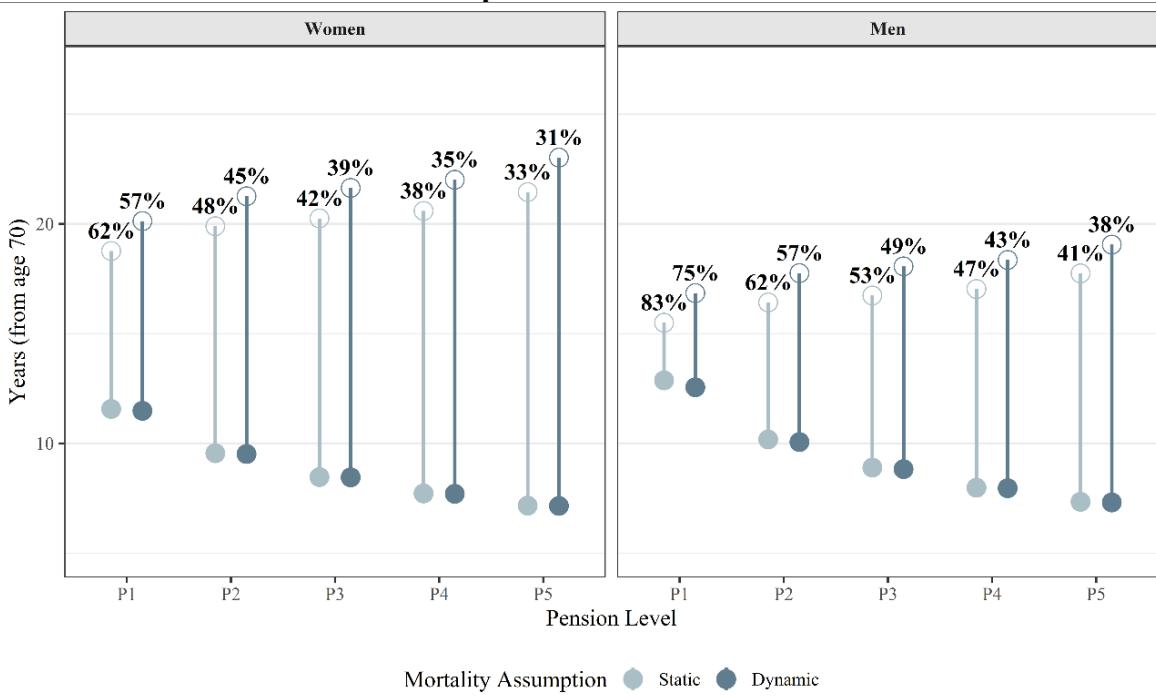
Figure 1 reports the baseline survival-horizon comparison for the benchmark profiles used in Section 4.1. The lower marker is the actuarial breakeven horizon, , and the upper marker is remaining life expectancy at effective retirement, . The vertical segment measures the survival margin after breakeven. Percentages report as a share of remaining life expectancy.
Figure 1 shows that the breakeven horizon absorbs a progressively smaller share of remaining life expectancy as the pension level increases. For women, this share falls from 62% under static mortality and 57% under dynamic mortality in P1 to 33% and 31%, respectively, in P5. For men, it falls from 83% and 75% in P1 to 41% and 38% in P5. Accordingly, the longer vertical segments observed at higher pension levels correspond to lower percentages, since a larger share of expected remaining lifetime lies beyond the breakeven point.
Figure 1. Remaining life expectancy and actuarial breakeven horizon by sex and pension level. Note: Benchmark: statutory retirement age 67, three-year delay, effective retirement at age 70, 1% real discount rate, and segmented pensioner mortality. Markers represent the breakeven horizon and remaining life expectancy; percentages report their ratio. Source: Own elaboration.
The final baseline diagnostic is the implicit real annual discount rate required to restore actuarial neutrality under exponential discounting. Table 6 reports this threshold for the same standard contribution regime used throughout the baseline analysis.
The threshold discount rates increase monotonically with pension entitlement and are higher for women than for men. Under dynamic mortality, the rate required to make the lump sum actuarially equivalent ranges from 7.33% in P1 to 14.53% in P5 for women, and from 5.79% to 13.58% for men. Thus, relatively high personal discount rates are required to overturn the common-discounting actuarial ranking, particularly for women and for middle- and high-pension profiles. The lowest threshold occurs for men in P1, the profile for which the statutory lump sum is closest to actuarial equivalence. These thresholds do not themselves explain observed choices; rather, they provide the profilespecific indifference rates that link the actuarial benchmark to the heterogeneousdiscounting analysis presented in Section 5.1.
Table 6: Implicit real annual discount rate required for actuarial neutrality Note: Thresholds are annual effective real discount rates. Source: Own elaboration.
| PL | Women | Men | ||
| r*(s) | r*(d) | r*(s) | r*(d) | |
| P1 | 6.93% | 7.33% | 5.17% | 5.79% |
| P2 | 9.58% | 9.88% | 7.96% | 8.45% |
| P3 | 11.42% | 11.68% | 9.90% | 10.34% |
| P4 | 12.96% | 13.20% | 11.57% | 11.96% |
| P5 | 14.32% | 14.53% | 13.26% | 13.58% |
The results are robust to replacing segmented pension-group mortality with generalpopulation mortality. General-population mortality raises L/APV modestly, but all reported ratios remain below one. The detailed mortality-basis comparison is therefore reported in the supplementary workbook. The profile-level results in this subsection establish the actuarial mechanism, but they do not by themselves identify the aggregate relevance of the lump-sum penalty.
4.2 Population-weighted relevance: MCVL evidence and actuarial tail-risk benchmark
The previous subsection established the profile-level actuarial benchmark. This subsection examines its quantitative relevance once the simulated profiles are weighted according to the characteristics of actual delayed retirees. Each 2024 MCVL administrative cell is matched to the corresponding simulated scenario by sex, pension band, contribution-formula regime, statutory ordinary retirement age, and completed delay duration. Cells with delays of seven years or more are assigned the seven-year simulation value. The complete cell-level matching is reported in the supplementary Excel workbook.
All population shares in Table 7 are computed within delayed-retirement records. The actuarial diagnostics use segmented dynamic mortality by sex and pension group and a 1% real discount rate as the main benchmark; static mortality is subsequently considered as a sensitivity check.
Table 7. Population-weighted MCVL evidence, lump-sum-component exposure, and actuarial tail-risk benchmark, 2024
| Dimension | Group | (%) | (1)-(2) | L/APV* | $T_{d}^{act}$ | ||
| Share | Observed (1) | $\pi_x$ (2) | |||||
| Overall | All | 100.00 | 24.02 | 15.62 | 8.40 | 0.512 | 10.84 |
| Sex | W | 35.22 | 23.28 | 9.33 | 13.95 | 0.472 | 10.40 |
| M | 64.78 | 24.42 | 19.04 | 5.38 | 0.534 | 11.07 | |
| Contribution formula | <44y6m | 70.79 | 21.70 | 14.61 | 7.08 | 0.501 | 10.55 |
| ≥44y6m | 29.21 | 29.65 | 18.05 | 11.60 | 0.539 | 11.52 | |
| Profile | P1 | 59.12 | 19.73 | 20.26 | -0.54 | 0.581 | 12.25 |
| P2 | 15.24 | 25.00 | 11.68 | 13.32 | 0.473 | 10.18 | |
| P3 | 6.93 | 40.00 | 9.41 | 30.59 | 0.428 | 9.06 | |
| P4 | 4.39 | 21.05 | 6.96 | 14.09 | 0.374 | 7.93 | |
| P5 | 14.32 | 33.87 | 6.27 | 27.60 | 0.353 | 7.45 | |
| Retirement age | 66 to <67 | 41.81 | 19.89 | 14.90 | 5.00 | 0.500 | 11.02 |
| 67 to <68 | 10.39 | 41.11 | 14.77 | 25.64 | 0.502 | 10.78 | |
| 68+ | 47.80 | 23.81 | 17.01 | 7.62 | 0.532 | 10.69 | |
| Delay | 1 year | 57.74 | 18.60 | 14.74 | 3.86 | 0.502 | 10.96 |
| 2 years | 18.59 | 36.02 | 15.34 | 20.68 | 0.512 | 10.79 | |
| 3+ years | 23.67 | 27.80 | 17.98 | 9.82 | 0.536 | 10.57 | |
Source: Own elaboration.
Observed lump-sum exposure combines the pure lump-sum and mixed options, as both provide immediate capital. This combined indicator should be interpreted cautiously. The mixed option retains part of the delayed-retirement incentive as a lifelong pension supplement and is therefore not economically equivalent to full commutation.
The key actuarial statistic is the population-weighted probability of dying before the breakeven horizon, , calculated as the weighted average of the profile-specific deathbefore-breakeven probabilities . This statistic is neither a predicted take-up rate nor an estimate of rational choice. It measures the ex-post probability that death occurs before the full annuity supplement recovers the corresponding statutory lump sum under objective survival probabilities. The comparison therefore applies most directly to the polar choice between the pure lump sum and the full annuity supplement. Its comparison with combined lump-sum exposure should be understood as a broader descriptive benchmark rather than as a like-for-like choice residual.
Table 7 brings these elements together. Column (1) reports the observed share of delayed retirees choosing an option with a lump-sum component, while column (2) reports the population-weighted actuarial tail-risk benchmark. The difference between them is therefore interpreted as an exposure gap. The final columns report the populationweighted fairness ratio, L/APV*, and the corresponding weighted actuarial breakeven horizon
At the aggregate level, 24.02% of delayed retirees chose an option containing a lumpsum component: 21.36% selected the pure lump sum and 2.66% the mixed option. Under dynamic segmented mortality, the population-weighted probability of death before actuarial breakeven is 15.62%. This produces a difference of 5.74 percentage points relative to pure lump-sum take-up and a broader exposure gap of 8.40 percentage points when the mixed option is also included. Under static mortality, the benchmark rises to 18.10%, reducing the corresponding differences to 3.26 and 5.92 percentage points. Objective survival tail risk alone therefore does not fully account for pure lump-sum takeup, although the remaining difference should not be interpreted as evidence of irrational choice.
The valuation columns show that the comparison does not involve a marginal actuarial difference. The population-weighted dynamic fairness ratio is 0.512, meaning that the statutory lump sum represents approximately 51% of the actuarial present value of the corresponding lifelong supplement. The weighted actuarial breakeven horizon is 10.84 years.
The sex decomposition reflects the role of longevity. Women account for 35.22% of delayed retirees and have a dynamic tail-risk benchmark of 9.33%, compared with combined lump-sum exposure of 23.28%. The corresponding figures for men are 19.04% and 24.42%. Because women have longer expected survival, the probability that full commutation becomes advantageous ex post is substantially lower, although observed exposure to immediate capital is similar across sexes.
The contribution-formula split points in the same direction. Retirees with at least 44 years and 6 months of contributions represent 29.21% of delayed-retirement records and have combined lump-sum exposure of 29.65%, compared with a dynamic tail-risk benchmark of 18.05%. For shorter contribution careers, the corresponding figures are 21.70% and 14.61%.
The pension-band decomposition links the population evidence to the distributional mechanism of the statutory formula. P1 is the dominant empirical group, accounting for 59.12% of delayed retirees. Its combined exposure rate, 19.73%, is close to the dynamic tail-risk benchmark of 20.26%. The benchmark subsequently falls to 6.27% in P5, while combined exposure reaches 40.00% in P3 and 33.87% in P5. Although some higherpension groups contain fewer observations, this pattern is consistent with the concavity of the statutory formula. The actuarial case for full commutation weakens as pension entitlement rises, while exposure to immediate capital does not decline accordingly.
Delay duration also matters. One- and two-year delays account for 76.33% of delayedretirement records. For one-year delays, combined exposure is 18.60%, compared with a dynamic tail-risk benchmark of 14.74%. For two-year delays, the corresponding figures are 36.03% and 15.34%. The observed difference is therefore concentrated partly in empirically important short-delay groups rather than only in remote long-delay scenarios.
Overall, the population-weighted results show that actuarial non-neutrality is not confined to isolated simulated profiles. At the same time, the comparison between combined exposure and the death-before-breakeven benchmark is descriptive, particularly because the mixed option retains an annuity component. The following sections therefore examine whether discounting heterogeneity, mortality pessimism, taxation, and other valuation considerations can help explain observed choices without treating the remaining difference as irrational behavior.
5. Extensions and Robustness
5.1 Behavioral valuation: discounting heterogeneity and mortality pessimism
Section 4.2 showed that objective death-before-breakeven risk does not fully account for observed pure lump-sum take-up. It also compared this benchmark with the broader exposure measure that includes the mixed option, while recognizing that the latter retains an annuity component. The narrower question addressed here is whether the valuation mechanisms represented in the model (heterogeneous exponential discounting, presentbiased or hyperbolic discounting, and subjective mortality pessimism) can make full commutation financially attractive for some profiles.
The analysis therefore remains at the level of financial valuation under alternative subjective assumptions. Accordingly, the results should not be interpreted as distinguishing between rational preference heterogeneity and behavioral bias. Instead, it asks how much the annuity-lump-sum comparison changes when retirees attach less value to future survival-contingent pension income than the baseline actuarial benchmark assumes. This framing follows the distinction introduced in Section 3 between actuarial non-neutrality, financial attractiveness under heterogeneous preferences, and welfare evaluation under maintained utility assumptions.
To keep the comparison internally consistent, Figure 2 and Tables 8 and 9 use the same benchmark: contribution histories below 44 years and 6 months, statutory ordinary retirement age 67, a three-year delay, effective retirement at age 70, segmented dynamic mortality by sex and pension group, and a 1% real exponential discount rate as the common-discounting baseline.
Figure 2 shows that present-oriented discounting raises the relative value of the lump sum, as expected. In the benchmark case, the exponential L/APV ratio ranges from 0.56 in P1 to 0.33 in P5 for women, and from 0.66 to 0.38 for men. The quasi-hyperbolic and hyperbolic specifications raise these ratios, especially at the lower end of the pension distribution, but they do not push any of the ten benchmark profiles above financial indifference. The strongest benchmark case remains men in P1, for whom the hyperbolic ratio reaches 0.91.
Figure 2: Fairness ratio under exponential, quasi-hyperbolic, and hyperbolic discounting Note: Benchmark: statutory age 67, three-year delay, claiming age 70, 1% real discount rate, standard contribution formula, and segmented dynamic mortality. The dashed line at L/APV = 1 denotes financial indifference. Source: Own elaboration.
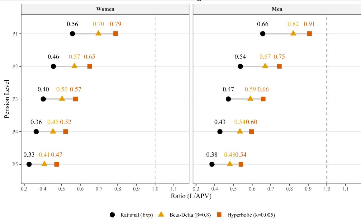
For contribution histories of 44 years and 6 months or longer, the statutory 10% uplift would raise each ratio proportionally. In this strongest case, the ratio would increase from 0.907 to approximately 0.998, effectively reaching financial indifference, while remaining below one for the other nine profiles.
Table 8 reports the heterogeneous-discounting results most directly relevant for interpreting whether subjective discounting can overturn the actuarial ranking for some retirees. When discounting is low, the median L/APV remains below one in all ten benchmark profiles. By contrast, under the central calibration, the median ratio exceeds one in 4 out of 10 profiles: P1 and P2 for both women and men. It also comes close to one for men in P3. The probability that an individual discount rate exceeds the profilespecific indifference rate is 67.1% for women in P1, 50.7% for women in P2, 78.3% for men in P1, and 59.5% for men in P2. These values show that, if subjective discount rates are high and dispersed, lump-sum valuation can be financially attractive for a nonnegligible subset of low-pension profiles.
The same table also shows where this explanation becomes less persuasive. Under the central calibration, the median ratio remains below one for P3-P5 across both genders. The median ratio remains below one for P3–P5 across both genders under the central calibration. In the high-discounting calibration, the median ratio exceeds one throughout the distribution, but that calibration is best interpreted as a strong sensitivity exercise rather than as the maintained benchmark. Heterogeneous discounting therefore cautions against describing the lump sum as universally unattractive, while preserving the baseline conclusion that the statutory formula is not actuarially neutral under common discounting and objective survival.
Table 8. Heterogeneous exponential discounting under segmented dynamic mortality
| Sex | Profile | Base L/APV | r* (%) | Median L/APV | P(ρ>r*) | ||
| Low | Central | High | Central (%) | ||||
| Women | P1 | 0.558 | 7.3 | 0.826 | 1.208* | 2.019* | 67.1 |
| P2 | 0.456 | 9.9 | 0.685 | 1.009* | 1.691* | 50.7 | |
| P3 | 0.402 | 11.7 | 0.606 | 0.897 | 1.514* | 41.2 | |
| P4 | 0.364 | 13.2 | 0.553 | 0.820 | 1.385* | 34.6 | |
| P5 | 0.326 | 14.5 | 0.505 | 0.754 | 1.290* | 29.7 | |
| Men | P1 | 0.657 | 5.8 | 0.939 | 1.322* | 2.148* | 78.3 |
| P2 | 0.537 | 8.4 | 0.774 | 1.109* | 1.791* | 59.5 | |
| P3 | 0.473 | 10.3 | 0.688 | 0.972 | 1.594* | 48.1 | |
| P4 | 0.428 | 12.0 | 0.622 | 0.887 | 1.460* | 39.9 | |
| P5 | 0.385 | 13.6 | 0.562 | 0.812 | 1.326* | 33.1 | |
| Source: Own elaboration. | |||||||
Table 9 reports the same indifference exercise for subjective survival beliefs across all five pension bands. The parameter is the survival-distortion factor required for the subjective actuarial value of the annuity supplement to equal the statutory lump sum; larger values imply stronger mortality pessimism. The table also reports the subjective life expectancy, , implied by , the actuarial breakeven horizon, , and the gap between the two, all measured in years from effective retirement.
Table 9. Mortality pessimism required for subjective indifference
| Sex | Profile | $\psi^*$ | $e_{70}^{subj}$ | $T_d^{act}$ | Gap |
| Women | P1 | 4.93 | 10.94 | 11.49 | -0.55 |
| P2 | 9.21 | 9.29 | 9.52 | -0.22 | |
| P3 | 12.33 | 8.28 | 8.46 | -0.18 | |
| P4 | 15.11 | 7.57 | 7.71 | -0.14 | |
| P5 | 16.47 | 7.03 | 7.15 | -0.12 | |
| Men | P1 | 2.49 | 10.99 | 12.56 | -1.57 |
| P2 | 4.03 | 9.33 | 10.06 | -0.74 | |
| P3 | 5.30 | 8.30 | 8.83 | -0.53 | |
| P4 | 6.64 | 7.58 | 7.96 | -0.38 | |
| P5 | 8.99 | 7.04 | 7.31 | -0.27 | |
| Source: Own elaboration. | |||||
Mortality pessimism works in the same direction as high discounting, but the required distortion varies sharply across profiles. For low-pension men, the indifference value is relatively moderate: equals 2.49 in P1, and the implied subjective life expectancy is 10.99 years compared with an actuarial breakeven horizon of 12.56 years. For women in P1, the required value is already higher, at 4.93. Moving up the pension distribution, the required distortion rises monotonically. In P5, reaches 16.47 for women and 8.99 for men. These values imply a strong compression of subjective survival probabilities, with subjective life expectancy converging closely to the breakeven horizon. The gap arises because subjective remaining life expectancy and the actuarial breakeven horizon summarize different objects. The indifference condition is based on the full discounted stream of survival-weighted annuity payments under the distorted subjective survival curve. By contrast, subjective life expectancy is the mean of that survival distribution, while the breakeven horizon identifies the time required for cumulative annuity payments to recover the lump sum. Consequently, present-value indifference does not imply equality between and . The remaining probability of surviving beyond the breakeven horizon contributes to the subjective value of the annuity and allows indifference to occur even when subjective life expectancy is somewhat shorter than the breakeven horizon.
The interpretation is therefore asymmetric. Mortality pessimism, private information about poor health, or a strong belief that one will not survive long enough to recover the annuity’s value may rationalize full commutation in some low-pension profiles, especially among men. By contrast, financial indifference among women and higherpension profiles requires much stronger subjective survival compression. This is consistent with the population-weighted evidence in Section 4.2: objective tail risk is most favorable to the lump sum at the lower end of the pension distribution and least favorable among longer-lived and higher-pension groups.
Overall, alternative time valuation and subjective survival beliefs narrow the gap identified in the actuarial analysis and can reverse the financial ranking in some lowpension profiles. This finding reinforces the distinction between actuarial non-neutrality and individual financial preference: a lump-sum choice need not be interpreted as a mistake merely because the statutory formula falls below actuarial equivalence under common discounting and objective survival. The effects are nevertheless uneven, being strongest among low-pension profiles and men and weakest among women and higher pension bands. The next subsection examines whether fiscal treatment and institutionalrisk exposure further increase the relative financial value of the lump sum.
5.2. Fiscal treatment and policy-risk sensitivity
This subsection considers two institutional channels that operate in the same direction: the tax treatment of the lump sum and the exposure of the deferred pension supplement to future policy risk. The purpose is not to redefine actuarial neutrality, which remains a gross valuation benchmark based on objective survival and common discounting, but to assess whether institutional frictions can make the lump-sum option financially more attractive for some representative profiles.
To keep the comparison aligned with the behavioral-valuation results in Section 5.1, Tables 10 and 11 use the same benchmark as Tables 8 and 9, while the full set of fiscal and policy-risk outputs for the expanded simulation grid is reported in the supplementary Excel workbook.
The fiscal channel reflects the fact that the deferred-retirement supplement is taxed gradually as ordinary pension income, whereas the lump sum is concentrated in the year of receipt. Under progressive personal income taxation, this timing difference may either penalize or favor commutation depending on the effective marginal tax rates applied to the two income increments. The Spanish tax treatment partly offsets this concentration effect because the lump sum may qualify for a 30% reduction in the taxable base, subject to regulatory ceilings. The simulation therefore compares gross valuation with net-of-tax valuation under the statutory 30% reduction, using the 2025 IRPF schedule and assuming no taxable income other than the pension.
Table 10 shows that favorable tax treatment improves the relative valuation of the lump sum in every benchmark profile. The increase is nevertheless modest in economic terms. For women, the net L/APV ratio rises from 0.558 to 0.589 in P1 and from 0.326 to 0.369 in P5. For men, it rises from 0.657 to 0.693 in P1 and from 0.385 to 0.435 in P5. The largest absolute increase is 0.068, for men in P4.
The supplementary fiscal module confirms that this conclusion extends beyond the ten benchmark profiles reported in Table 10. Under the dynamic segmented benchmark, the lump-sum tax rate required to restore net actuarial neutrality lies outside the feasible [0,1] range in 275 of the 280 profiles. The few feasible cases are confined to low-pension men with long delays.
Table 10. Fiscal impact on L/APV and actuarial breakeven, segmented dynamic mortality
| Sex | Profile | $\rho_{gross}$ | Net Ratio ( $\vartheta = 0.30$ ) | Change | $T_d^{act}$ | |
| Gross | Net | |||||
| Women | P1 | 0.558 | 0.589 | 0.031 | 11.49 | 12.27 |
| P2 | 0.456 | 0.498 | 0.042 | 9.52 | 10.49 | |
| P3 | 0.402 | 0.424 | 0.022 | 8.46 | 8.96 | |
| P4 | 0.364 | 0.421 | 0.058 | 7.71 | 9.00 | |
| P5 | 0.326 | 0.369 | 0.042 | 7.15 | 8.15 | |
| Men | P1 | 0.657 | 0.693 | 0.036 | 12.56 | 13.50 |
| P2 | 0.537 | 0.586 | 0.049 | 10.06 | 11.21 | |
| P3 | 0.473 | 0.499 | 0.026 | 8.83 | 9.39 | |
| P4 | 0.428 | 0.496 | 0.068 | 7.96 | 9.43 | |
| P5 | 0.385 | 0.435 | 0.050 | 7.31 | 8.36 | |
| Source: Own elaboration | ||||||
The breakeven interpretation is similar. With the statutory reduction, the after-tax financial breakeven horizon increases relative to the gross benchmark because the net value of the lump sum rises relative to the net annuity supplement. For example, the horizon increases from 11.49 to 12.27 years for women in P1, and from 12.56 to 13.50 years for men in P1. These changes matter for valuation, but they do not move the breakeven horizon beyond remaining life expectancy in any of the benchmark profiles. Without the 30% reduction, the progressive tax schedule lowers the net L/APV ratio in all profiles; those results are reported in the supplementary workbook.
Table 11 applies the policy-risk stress test defined in Section 3.2.4. The exercise should be read narrowly: it captures exposure of the deferred supplement to one adverse pensionrule scenario, while recognizing that an immediate lump sum is no longer protected by pension indexation and remains exposed to reinvestment and inflation risk. The table reports how this institutional-risk adjustment changes the L/APV ratio under exponential, quasi-hyperbolic, and hyperbolic discounting, with the final column also incorporating the statutory 30% tax reduction.
Table 11. Policy-risk effects on L/APV under alternative discounting specifications and favorable tax treatment, segmented dynamic mortality Source: Own elaboration
| Sex | Profile | Discounting | ||||
| Exponential | Quasi Hyp. | Hyperbolic | ||||
| No Risk | Risk | Risk | Risk | Risk + Tax | ||
| Women | P1 | 0.558 | 0.665 | 0.830 | 0.927 | 0.978 |
| P2 | 0.456 | 0.545 | 0.680 | 0.765 | 0.836 | |
| P3 | 0.402 | 0.481 | 0.600 | 0.678 | 0.715 | |
| P4 | 0.364 | 0.435 | 0.544 | 0.616 | 0.714 | |
| P5 | 0.326 | 0.392 | 0.490 | 0.560 | 0.633 | |
| Men | P1 | 0.657 | 0.776 | 0.969 | 1.056* | 1.114* |
| P2 | 0.537 | 0.636 | 0.794 | 0.871 | 0.951 | |
| P3 | 0.473 | 0.561 | 0.701 | 0.770 | 0.812 | |
| P4 | 0.428 | 0.508 | 0.634 | 0.698 | 0.809 | |
| P5 | 0.385 | 0.458 | 0.572 | 0.633 | 0.715 | |
| Source: Own elaboration | ||||||
Under exponential discounting, policy risk raises the L/APV ratio in every profile, but the ratio remains below one throughout the benchmark distribution. For women, the policyrisk ratio ranges from 0.665 in P1 to 0.392 in P5. For men, it ranges from 0.776 in P1 to 0.458 in P5. Thus, policy risk materially compresses the actuarial gap, but it does not by itself restore financial equivalence.
The effect becomes stronger when policy risk is combined with present-oriented valuation. Under the quasi-hyperbolic specification, men in P1 reach 0.969, close to indifference, while all other profiles remain below one. Under hyperbolic discounting, men in P1 cross the indifference threshold, with L/APV equal to 1.056. This is the only benchmark profile in which policy risk combined with non-exponential discounting makes the lump sum financially preferable before taxes.
The final column adds the statutory 30% lump-sum tax reduction to the hyperbolic policyrisk valuation by applying the profile-specific fiscal scaling factor from Table 10. This combined stress test is the most favorable valuation environment considered in the main text. It raises the ratio to 1.114 for men in P1 and to 0.978 for women in P1; men in P2 also move close to indifference, at 0.951. The remaining profiles continue to lie below one, and the gap remains particularly large in the higher pension bands.
Fiscal treatment and policy risk therefore compress the actuarial gap and, when combined with present-oriented discounting, can bring the lump sum close to or above indifference for low-pension men. However, these institutional channels do not overturn the broader distributional pattern: the gap remains largest for women and for higher pension bands, where longevity and the concavity of the lump-sum formula make the annuity supplement most valuable.
5.3. Combined assessment of modelled channels
Sections 5.1 and 5.2 evaluate the main non-baseline channels one at a time: heterogeneous or non-exponential discounting, subjective survival beliefs, favorable tax treatment, and policy risk. These mechanisms need not operate in isolation. A retiree who chooses the lump sum may simultaneously place a high value on immediate liquidity, face favorable tax treatment, and attach value to avoiding long-run institutional risk. This subsection therefore assesses how far the modelled channels go when considered jointly.
The exercise should be interpreted carefully. A cell with L/APV ≥ 1 under a combined scenario is a profile in which the statutory lump sum is financially at least as valuable as the annuity supplement under the assumptions of that scenario. It is not a predicted takeup rate. Conversely, a profile with L/APV below one should not be read as evidence of irrational choice, since the model does not capture unobserved health, liquidity, household, and bequest-related factors that may influence individual decisions. The combined exercise is therefore a bridge between the actuarial results and the later discussion of observed take-up.
Table 12 reports the combined assessment for the 280 dynamic segmented simulation profiles defined by sex, pension band, contribution-formula regime, statutory ordinary age, and delay duration. The contribution-formula dimension includes both careers below the 44-year-and-6-month threshold and longer careers receiving the statutory 10% lumpsum uplift. It also reports the corresponding 2024 MCVL-weighted results, using the administrative cell weights introduced in Section 3.1.3. The scenarios apply the policyrisk stress test and the favorable tax treatment defined in Section 5.2. The final column reports the contribution, in percentage points, to aggregate lump-or-mixed take-up from profiles in which the relevant scenario produces L/APV ≥ 1.
| Valuation environment | % of Cells with L/APV ≥ 1 | L/APV | MCVL % with L/APV ≥ 1 | Observed take-up% | |
| Mean grid | MCVL-weighted | ||||
| Gross exponential baseline | 0.00 | 0.485 | 0.512 | 0.00 | 0.0 |
| Favorable tax treatment | 0.00 | 0.526 | 0.555 | 0.00 | 0.0 |
| Policy risk, exponential | 0.36 | 0.576 | 0.611 | 0.00 | 0.0 |
| Policy risk + Quasi | 6.79 | 0.719 | 0.763 | 3.23 | 1.0 |
| Policy risk + hyperbolic | 13.93 | 0.798 | 0.857 | 18.94 | 4.6 |
| Policy risk + hyp. + tax | 21.43 | 0.867 | 0.929 | 39.38 | 8.0 |
| Source: Own elaboration | |||||
The combined scenarios in Table 12 include only channels that generate a single celllevel L/APV ratio and can therefore be aggregated transparently using the MCVL weights. The exercise does not attempt to assign unobserved preference or belief heterogeneity to administrative cells. In particular, subjective survival beliefs are left as a separate sensitivity, since mapping them into the MCVL structure would require assumptions not observed in the data. The table should therefore be read as a profile-level benchmark rather than as an exhaustive representation of individual choice mechanisms.
The table confirms that neither taxation nor policy risk is sufficient on its own to overturn the baseline ranking in a population-relevant way. Favorable tax treatment raises the MCVL-weighted L/APV ratio from 0.512 to 0.555, but no simulated profile reaches financial indifference. Policy risk under exponential discounting raises the MCVLweighted ratio to 0.611, but only one of the 280 simulated profiles crosses L/APV = 1, and that profile has no weight in the observed MCVL profile structure.
The picture changes once policy risk is combined with present-oriented valuation. Under the quasi-hyperbolic specification, 19 of the 280 profiles reach or exceed financial indifference, but these profiles account for only 3.23% of the MCVL-weighted delayedretirement population. Under hyperbolic discounting, the number rises to 39 profiles and the population-weighted share to 18.94%. Adding favorable tax treatment produces the most lump-sum-favorable environment considered in the main text: 60 profiles reach L/APV ≥ 1, representing 21.43% of the simulation grid and 39.38% of the 2024 delayedretirement population.
This result shows that the combined channels can make lump-sum commutation financially defensible for a meaningful set of empirically relevant profiles under the maintained assumptions. The MCVL-weighted share exceeds the unweighted cell share because favorable outcomes are concentrated in low-pension profiles, particularly P1, which represent a large proportion of observed delayed retirees. The result therefore supports a more nuanced interpretation of observed take-up, without implying that the model predicts individual choices.
The combined scenario nevertheless leaves much of the baseline valuation gap intact. Even in the most favorable specification, the MCVL-weighted L/APV ratio remains below one, at 0.929. Profiles reaching L/APV ≥ 1 contribute 8.0 percentage points to the aggregate lump-or-mixed take-up rate of 24.02%, or approximately one-third of observed take-up. This does not mean that the remaining choices are irrational; rather, their valuation may reflect individual characteristics and motives that cannot be observed in the cell-level exercise.
Overall, the combined assessment supports a two-sided interpretation. The statutory formula remains non-neutral under baseline valuation and for most profiles, but commutation becomes financially defensible for a relevant subset once policy risk, present-oriented discounting, and favorable tax treatment are combined. The policy concern is therefore not that every lump-sum choice is mistaken, but that the distance between statutory compensation and the value of the foregone annuity varies systematically across groups.
6. Welfare Evaluation
This section reports the certainty-equivalent results generated by the welfare framework defined in Section 3.2.5. The exercise asks how surrendering the lifelong supplement changes equivalent monthly consumption when pension income is used as a proxy for retirement consumption.
Table 13 reports a compact summary for the dynamic segmented mortality profiles. The unweighted mean describes the complete simulation grid, while the population-weighted columns translate the same welfare metric into the empirical structure of delayedretirement records observed in the 2024 MCVL.
Table 13. Certainty-equivalent gap under CRRA preferences, dynamic segmented mortality
| Group | MCVL share (%) | Unweighted mean CE gap (%) | MCVL-weighted CE gap (%) | MCVL-weighted monthly CE gap (EUR) |
| All cells | 100.00 | 5.86 | 3.00 | 71.4 |
| Women | 35.22 | 6.50 | 3.48 | 73.5 |
| Men | 64.78 | 5.23 | 2.73 | 70.2 |
| P1 | 59.12 | 3.33 | 2.33 | 32.1 |
| P2 | 15.24 | 5.18 | 2.67 | 52.7 |
| P3 | 6.93 | 6.16 | 3.78 | 102.5 |
| P4 | 4.39 | 7.11 | 4.34 | 145.7 |
| P5 | 14.32 | 7.52 | 5.32 | 215.7 |
| 1-year delay | 57.74 | 2.00 | 1.69 | 32.8 |
| 2-year delay | 18.59 | 3.72 | 3.16 | 69.6 |
| 3-5-year delays | 16.97 | 6.25 | 6.02 | 174.9 |
| 6-7-year delays | 6.70 | 8.28 | 6.18 | 146.5 |
Note: The central calibration uses CRRA preferences with γ = 2 and a 1% annual real exponential discount rate. The relative CE gap is calculated as defined in Equation (23). Population weights correspond to the 2024 MCVL.
Source: Own elaboration.
The table gives a more cautious reading than the unweighted profile-level results alone. Across the full dynamic segmented simulation grid, the mean relative certaintyequivalent gap is 5.86%. Once the results are weighted by the 2024 MCVL distribution, the mean relative gap falls to 3.00%, and the mean monthly certainty-equivalent difference is EUR 71.4. This reduction is compositional: observed delayed retirees are concentrated in lower-pension and shorter-delay profiles, where the conditional welfare gap is smaller.
The distributional pattern nevertheless remains visible. Under the maintained CRRA specification, the MCVL-weighted relative gap is higher for women than for men, reflecting the greater value of longevity insurance when expected survival is longer. It also rises with pension level, from 2.33% in P1 to 5.32% in P5, and with delay duration. The gap is 1.69% for one-year delays, which account for 57.74% of observed delayedretirement records, but rises to about 6% for delays of three years or more. These patterns are consistent with the actuarial gradient documented earlier, but they should not be interpreted as unconditional welfare losses for all individuals in those groups. They describe the certainty-equivalent implication of the statutory commutation formula within the assumed consumption and utility framework.
Figure 3 complements Table 13 by displaying the joint distribution of certainty-equivalent gaps and population weights for selected pension bands P1, P3, and P5. Bubble colour represents the MCVL-weighted relative certainty-equivalent gap, while bubble area represents the corresponding share of 2024 delayed-retirement records. The largest gaps are concentrated in higher-pension and longer-delay profiles, whereas the greatest population weights occur among lower-pension and shorter-delay profiles, particularly men in P1. Women generally exhibit larger gaps than comparable male profiles. This composition explains why the MCVL-weighted welfare gap is lower than the unweighted simulation-grid average.
Figure 3. Certainty-equivalent gaps and MCVL population shares by sex, selected pension band, and delay duration Note: P1, P3, and P5 are shown for readability. Bubble colour represents the relative certaintyequivalent gap and bubble area the corresponding share of 2024 MCVL delayed-retirement records. Values are aggregated across statutory-age and contribution-formula cells using MCVL weights.
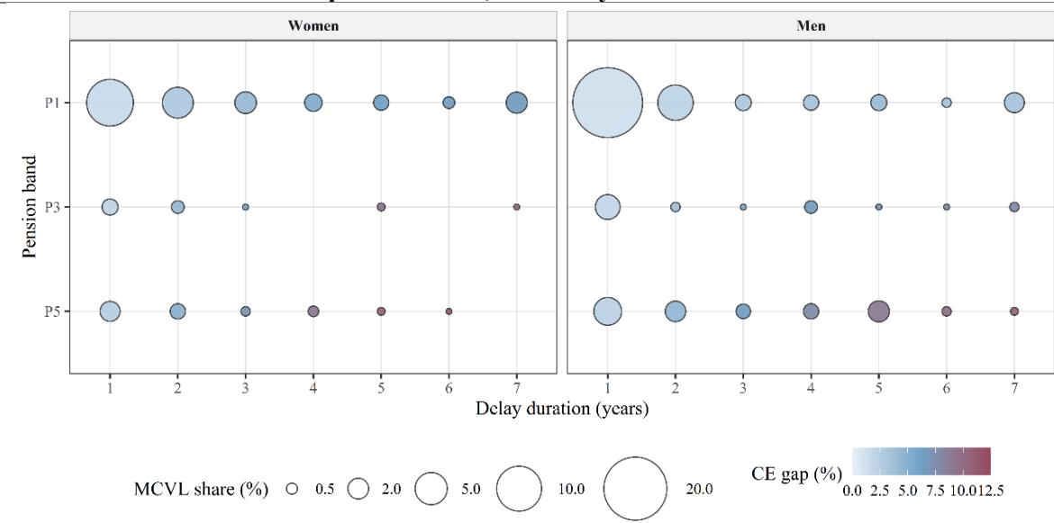
The welfare-equivalent lump-sum results point in the same direction. Under the central CRRA calibration and dynamic segmented mortality, the statutory lump sum is below the welfare-equivalent lump sum in all 280 simulated profiles. Measured relative to the statutory payment, the welfare-equivalent amount is higher by a median of 92.5% and a mean of 94.3%. When γ varies from 1.5 to 4.0, the median excess declines from 95.9% to 85.9%. At � = 3 and � = 4, only one of the 280 profiles marginally reverses the ranking. The broad result is therefore not driven by the central risk-aversion parameter, although its magnitude remains conditional on the maintained welfare framework.
The central welfare analysis uses CRRA preferences, under which welfare depends on proportional changes in total consumption. This specification may not fully capture the importance of preserving lifelong pension income when consumption is close to a minimum living standard. We therefore use Stone–Geary preferences as a robustness
Note: The Stone–Geary specification uses a subsistence floor equal to twice the 2025 noncontributory pension benchmark. Differences are calculated relative to the corresponding CRRA estimates in Table 13. All other assumptions and definitions are unchanged. Source: Own elaboration
exercise. By defining utility over consumption above a subsistence floor, this specification gives greater weight to income losses affecting profiles with limited consumption above that threshold. Table 14 reports the Stone–Geary results using a subsistence floor equal to twice the 2025 non-contributory pension benchmark and compares them directly with the corresponding CRRA estimates in Table 13.
The Stone–Geary specification produces results very close to the central CRRA estimates. The aggregate MCVL-weighted gap increases only slightly, from 3.00% to 3.06%, while the corresponding monthly gap declines from EUR 71.4 to EUR 70.0. Differences are similarly small across sex and pension groups. The principal distributional patterns therefore remain unchanged: the relative gap is larger for women than for men and rises from 2.41% in P1 to 5.34% in P5. It also generally increases with delay duration. The largest departure from the CRRA results occurs for delays of six to seven years, although these profiles represent only 6.70% of delayed-retirement records.
Table 14. Comparison of certainty-equivalent gaps under CRRA and Stone–Geary preferences
| Group | Stone-Geary MCVL-weighted CE gap (%) | Dif. from CRRA (pp) | Stone-Geary monthly CE gap (EUR) | Dif. from CRRA (EUR) |
| All cells | 3.06 | +0.06 | 70.0 | -1.4 |
| Women | 3.61 | +0.13 | 72.6 | -0.9 |
| Men | 2.76 | +0.03 | 68.6 | -1.6 |
| P1 | 2.41 | +0.08 | 30.8 | -1.3 |
| P2 | 2.71 | +0.04 | 51.5 | -1.2 |
| P3 | 3.80 | +0.02 | 100.7 | -1.8 |
| P4 | 4.37 | +0.03 | 144.2 | -1.5 |
| P5 | 5.34 | +0.02 | 213.9 | -1.8 |
| 1-year delay | 1.77 | +0.08 | 32.6 | -0.2 |
| 2-year delay | 3.26 | +0.10 | 68.6 | -1.0 |
| 3-5-year delays | 6.08 | +0.06 | 172.0 | -2.9 |
| 6-7-year delays | 5.94 | -0.24 | 138.3 | -8.2 |
The annuity produces the higher certainty equivalent in 279 of the 280 simulated profiles. The only reversal concerns a male P1 profile with a long contribution career, statutory age 67, and a seven-year delay. Using the 2025 non-contributory pension itself, rather than twice that amount, as the subsistence floor produces virtually identical aggregate results: an MCVL-weighted gap of 2.97%, a monthly gap of EUR 70.2, and the same 279-to-1 profile ranking.
Overall, the welfare results are consistent with the actuarial non-neutrality documented earlier, but they do not independently establish that observed lump-sum choices reduce individual welfare. Under both CRRA and subsistence-sensitive preferences, population weighting reduces the average certainty-equivalent gap to approximately 3%, without altering the main distributional gradients. These results should therefore be interpreted as conditional simulations of the statutory exchange rather than as a general welfare ranking of actual retirees’ choices.
7. Discussion and Policy Implications
The discussion focuses on the implications of actuarial non-neutrality for commutation design and on the distinction between the statutory terms of the exchange and the circumstances that may shape individual choices. Actuarial neutrality is used here as a valuation benchmark for the statutory exchange, rather than as a sufficient condition for individual welfare or as a claim about the stated objectives of Law 21/2021. In the Spanish case, the deviation from neutrality arises mainly from the interaction between the statutory formula and heterogeneous longevity. The annuity supplement scales proportionally with pension entitlement and is paid for life, whereas the lump sum follows a concave schedule and does not explicitly incorporate survival prospects. Consequently, women receive less favorable actuarial terms because of their longer expected survival, while higher-pension profiles are additionally affected by the sub-proportional growth of the lump sum.
The MCVL evidence qualifies the population relevance of this pattern. The largest actuarial deviations occur among longer-lived, higher-pension profiles, whereas observed delayed retirees are concentrated in shorter delays and lower pension bands, where the gaps tend to be smaller. Population weighting therefore moderates the aggregate magnitude of the actuarial and welfare differences without altering the underlying nonneutrality of the formula. The relevant policy issue is that a formally uniform commutation rule produces different economic terms across groups while being presented as part of the same delayed-retirement choice architecture.
Observed lump-sum take-up should nevertheless not be interpreted as evidence of irrationality. Heterogeneous discounting, favorable tax treatment, subjective survival pessimism, and policy-risk concerns can increase the relative value of immediate capital and, for some profiles, make the lump sum financially defensible. This is consistent with the annuity and decumulation literature, which identifies liquidity needs, precautionary motives, bequest preferences, control over wealth, framing effects, and subjective survival beliefs as possible reasons for preferring lump sums or flexible withdrawals (Bütler & Teppa, 2007; Lockwood, 2012; Beshears et al., 2014; Brown et al., 2016; O’Dea & Sturrock, 2023). Household balance sheets, private health information, financial advice, long-term care risk, and confidence in future pension commitments may also affect individual decisions but are not observed in the present framework.
The welfare analysis should be interpreted within the same distinction. The certaintyequivalent exercise captures the longevity-insurance value of the annuity supplement within a standard expected-utility framework (Yaari, 1965; Davidoff et al., 2005). Its results are conditional, however, on the maintained assumptions concerning preferences, consumption and use of the lump sum. They complement the actuarial analysis but do not provide a complete normative ranking of observed choices. A lump sum with a lower actuarial value may still improve individual welfare when unobserved factors such as those discussed above play a sufficiently important role.
The comparative evidence also helps clarify what is distinctive about the Spanish arrangement. In most advanced public pension systems, delayed claiming is rewarded primarily through a permanent increase in lifetime pension benefits. Notional definedcontribution systems such as those of Sweden, Italy, Latvia and Norway similarly incorporate delayed claiming into the conversion of accumulated pension rights into lifetime income. Where lump-sum mechanisms have existed, as in the United Kingdom and Australia, they have generally played a more limited role and have not operated as permanent central substitutes for actuarially adjusted pension increments (Department for
Work and Pensions, 2026; Australian Government, 2026). Belgium provides only a partial comparison because its retirement bonus is supplementary rather than a general commutation of a life-contingent supplement (Service fédéral des Pensions, 2024a, 2024b; Çetin & Jousten, 2025).
Spain is therefore distinctive because immediate capital is offered as a salient statutory alternative within the core delayed-retirement incentive. At the same time, comparatively high replacement rates and statutory pension indexation already provide substantial longevity and inflation insurance. The lump-sum option may consequently be understood as a liquidity and flexibility mechanism rather than as an alternative source of old-age insurance. This makes its calibration particularly important: flexibility introduced through non-neutral commutation terms has unequal consequences across pension and longevity profiles.
The fiscal implications should also be distinguished from both actuarial valuation and individual choice. Under the common mortality and discounting assumptions used in the baseline, the statutory lump sum is generally below the actuarial present value of the foregone supplement. If lump-sum recipients had survival prospects similar to those represented by these assumptions, commutation would reduce expected future pension liabilities by replacing a life-contingent obligation with a smaller immediate payment. The actual fiscal effect, however, depends on selection into the lump-sum option. Individuals with shorter expected lifetimes, potentially informed by private health information, may be more likely to choose immediate capital. When death occurs before the actuarial breakeven horizon, the lump sum exceeds the realized value of the supplement that would otherwise have been paid. The budgetary effect therefore depends on the conditional survival distribution of actual recipients, which is not observed in the present analysis. The estimated net savings of 0.17% of GDP reported by De la Fuente (2023) provide a separate budgetary assessment, but they should not be interpreted as direct evidence that commutation necessarily transfers pension value from retirees to the Social Security system.
These findings support two related policy responses. First, information provided at the point of choice could include the statutory lump sum, the actuarial value of the foregone supplement, the breakeven survival horizon, and the lump-sum amount required for equivalence under clearly stated assumptions (Ventura-Marco et al., 2023; Vidal-Meliá et al., 2024). Second, if commutation is retained, the actuarial present value of the foregone supplement could serve as a transparent reference value for calibrating the statutory payment. This does not require exact equivalence. A redesigned formula could set the lump sum as an explicit proportion of that reference value, with a conversion coefficient equal or close to one when approximate neutrality is intended, or below one when policymakers deliberately attach a discount to the liquidity and flexibility provided by immediate capital. Cash-for-care arrangements in long-term-care systems illustrate more generally that cash and in-kind alternatives need not be assigned identical monetary values when they provide different degrees of discretion and involve different modes of provision (Da Roit & Moreno-Fuentes, 2019). Although the analogy is not exact, since pension commutation involves surrendering accrued life-contingent income, it shows that a transparent discount relative to the actuarial benchmark need not be intrinsically inappropriate. Any departure from the actuarial benchmark should therefore be explicitly justified, periodically reviewed, and disclosed to claimants.
The analysis has several limitations. It does not estimate a structural model of delayedretirement choice, observe individual health, wealth, household composition, financial literacy or bequest motives, or model endogenous retirement timing and generalequilibrium labour-supply responses. The behavioral, fiscal, policy-risk and welfare exercises should therefore be understood as sensitivity analyses around the actuarial benchmark. These limitations restrict conclusions about individual choices, but not the assessment of the statutory commutation formula itself.
8. Conclusions
This paper shows that the Spanish statutory lump-sum formula does not generally provide an actuarially neutral exchange for the foregone delayed-retirement supplement. The gap varies systematically across profiles because the lump sum increases less than proportionally with pension entitlement, whereas the value of the annuity supplement rises with both pension amount and expected survival. It is therefore larger for women and higher-pension profiles. MCVL weighting moderates but does not overturn this result, since delayed retirees are concentrated in shorter delays and lower pension bands, where the gaps tend to be smaller.
These findings concern the statutory terms of commutation, not the rationality of observed choices. Preference heterogeneity, subjective survival beliefs, taxation, and policy risk can make immediate capital financially defensible for some profiles, while the welfare results remain conditional on the maintained expected-utility assumptions. Actuarial non-neutrality should therefore be distinguished from both individual financial attractiveness and welfare.
The main policy implication is to improve transparency and review the calibration of the commutation formula, rather than to eliminate flexibility. Retirees should receive comparable information on the statutory lump sum, the actuarial value of the foregone supplement, and the breakeven survival horizon. If commutation deliberately departs from neutrality, the extent and distribution of that departure should be made explicit. More broadly, the Spanish case shows that expanding pension choice requires attention not only to the options offered, but also to the valuation rule governing the exchange between immediate capital and lifetime income.
9. References
- Achury, C., Hubar, S., & Koulovatianos, C. (2012). Saving rates and portfolio choice with subsistence consumption. Review of Economic Dynamics, 15(1), 108–126. https://doi.org/10.1016/j.red.2011.01.002
- Andersen, S., Harrison, G. W., Lau, M. I., & Rutström, E. E. (2008). Eliciting risk and time preferences. Econometrica, 76(3), 583–618. https://doi.org/10.1111/j.1468- 0262.2008.00848.x
- Ashraf, N., Karlan, D., & Yin, W. (2006). Tying Odysseus to the mast: Evidence from a commitment savings product in the Philippines. Quarterly Journal of Economics, 121(2), 635–672. https://doi.org/10.1162/qjec.2006.121.2.635
- Australian Government, Department of Social Services. (2026). Pension Bonus Scheme. Social Security Guide. Retrieved June 12, 2026, from https://guides.dss.gov.au/socialsecurity-guide/3/4/7/100
- Bachmann, K., Lot, A., Xu, X., & Hens, T. (2023). Experimental research on retirement decision-making: Evidence from replications. Journal of Banking & Finance, 152, 106851. https://doi.org/10.1016/j.jbankfin.2023.106851
- Beshears, J., Choi, J. J., Laibson, D., Madrian, B. C., & Zeldes, S. P. (2014). What makes annuitization more appealing? Journal of Public Economics, 116, 2–16. https://doi.org/10.1016/j.jpubeco.2013.05.007
- Bockweg, C., Ponds, E. H. M., Steenbeek, O., & Vonken, J. (2018). Framing and the annuitization decision: Experimental evidence from a Dutch pension fund. Journal of Pension Economics and Finance, 17(3), 385–417. https://doi.org/10.1017/S147474721700018X
- Brown, J. R., Kapteyn, A., & Mitchell, O. S. (2016). Framing and claiming: How information-framing affects expected Social Security claiming behavior. Journal of Risk and Insurance, 83(1), 139–162. https://doi.org/10.1111/j.1539-6975.2013.12004.x
Este texto se ha extraído automáticamente del documento original. Para citarlo o leerlo con su maquetación, descargue el PDF.
Descargar en PDF