Returns to Caring? Health and Wellbeing Effects of Subsidized Long-Term Care
JOAN COSTA-FONT
SERGI JIMÉNEZ-MARTÍN
CRISTINA VILAPLANA-PRIETO
Estudios sobre la Economía Española 2026/30
Septiembre 2026
fedea
Las opiniones recogidas en este documento son las de sus autores y no coinciden necesariamente con las de Fedea.
Joan Costa-Fonta, Sergi Jiménez-Martínb and Cristina Vilaplana-Prietoc aLondon School of Economics and Political Science (LSE), CESIfo & IZA bUniversitat Pompeu Fabra, Barcelona School of Economics (BSE) and FEDEA cUniversity of Murcia
Abstract
We estimate the health and wellbeing effects of subsidized access to long-term care (LTC). Our analysis exploits the staggered implementation of Spain’s 2007 System of Autonomy and Care for Dependent People (SAAD), which expanded publicly funded and universal LTC subsidies and supports, as well as its subsequent reform. Using two decades worth of administrative and survey data and leveraging exogenous regional and individual-level variation in program exposure, we find that access to SAAD benefits reduces the care receiver’s depressive symptoms by about 1 percentage point, increases its survival probability by 2.6–3 percentage points, and raises its life satisfaction by 0.24–0.50 scale points. Cost-effectiveness estimates indicate that the implied cost per quality-adjusted life year (QALY) gained lies below commonly accepted efficiency thresholds for public health spending in Europe. These findings document sizeable health returns and efficiency gains from publicly subsidized LTC provision.
Keywords: long-term care subsidies, long-term care supports, old age care, Spain, mortality, cost per QALY, survival, mental health, and life satisfaction.
JEL: I18, J14, J16.
ℵContract author: Joan Costa-Font, Department of Health Policy, London School of Economics. E-mail; j.costafont@lse.ac.uk. We acknowledge financial help from the Agencia Estatal de Investigación project PID2023- 147602OB-I00. Sergi Jiménez acknowledges financial support from the Spanish Ministry of Economy and Competitiveness, through the Severo Ochoa Programme for Centers of Excellence in R&D (CEX2024-001476- S). We thank the seminar participants who have taken part in the Ageing@ LSE seminar, and the International Long Term Care Conference in Bilbao, Economics Department at UPF Barcelona, Erasmus University Department of Applied Economics, the Gateway for Ageing, RWI Essen, and Economics Department at Hagen University.
1. Introduction
Timely access to care can prevent episodes of ill health, mental disorders, and even premature death, whereas the alternative is often enduring unmet care needs. Although access to care, at times can reducing hospitalisations (Costa-Font et al, 2018) and improve the lives of caregivers and their families (Coe and van Houtven, 2009; Costa-Font and Vilaplana, 2022b; Costa-Font et al, 2023a), there are potentially long-term effects in care receivers health status, wellbeing and survival which we still know little about.
Long-term care (LTC) programs remain comparatively underfunded and less developed than healthcare programs. This underfunding can give rise to spillovers affecting care recipients’ health and wellbeing, caregivers’ outcomes, and broader economic dynamics (Barber et al., 2021; Angrisani et al., 2022; Costa-Font and Vilaplana-Prieto, 2022a; Chen and Zhao, 2023; Coe et al., 2023). However, while in many European health systems, programme subsidisation is guided by cost-effectiveness thresholds, such thresholds are not extended to LTC programs. Hence, identifying the causal effects of LTC programmes on recipients’ health using exogenous variation from LTC reform is central to making subsidisation decisions by benchmarking LTC programs them against other health interventions.
To date, most attempts to measure the health effects of LTC programs do not fully account its comprehensive range of effects on the health and wellbeing of care receivers, or when they do, this evidence does not result from causal estimates. The exception is Yang et al (2016), who employs care-related quality of life measures using the cross-sectional Adult Social Care Survey, but their estimates are descriptive and do not result from an exogenous variation. Other descriptive studies have examined the correlation of long-term care and some health outcomes. Tamiya et al. (2011), using a national survey before and after the start of the LTC program in Japan (which only offered supports), document no evidence on either the subjective health status of elderly care recipients or their ability to perform daily tasks. In contrast, Kuzuya et al. (2006) document that the more frequent use of day care services led to lower mortality in frail adults living in the community. So far, most studies have focused on some partial measures of mental health or mortality alone, mainly drawing on instrumental variable designs, as well as spillover effects on caregivers’ wellbeing, but (with the notable exception of Lei et al. (2025)) limited attention has been placed on policy intervention providing quai-experimental evidence.
Some studies have looked at partial effects by exploiting different instrumental strategies (e.g., daughters’ composition in the household, prices of formal care or cross-country legislation to measure the effect of care eligibility) on measures of mental health, quality of life and the presence depressive symptoms (Carrino et al, 2025). However, to date, there is limited evidence on the broader health and wellbeing effects resulting from interventions expanding LTC subsidies and supports. This gap partly is explained by the fact that long-term health impacts require time to exhibt health and wellbeing effects, making them difficult to capture in shorter evaluation windows or instrumental variable strategies. Moreover, existing studies generally do not typically provide estimates of the cost-effectiveness of affordable access to LTC.
This paper draws on quasi-experimental evidence from Spain, and more specifically on the wide and across the board expansion of access to LTC subsidies (e.g., care allowances) and supports (e.g., home care program) after the introduction of System of Autonomy and Attention to Dependent People (SAAD) in Spain, between 2007 to 2020, which extended both the subsidies and support to individuals in need of care, that otherwise would have gone with unmet needs. The specific focus in Spain is important because before the reform, the availability of subsidies and supports was very scarce, means tested and typically, the expectation was that individuals would receive informal care or undergo unmet needs which might, in turn, depress their health and wellbeing in later life. This study exploits almost two decades worth of regional and individual variation of the access to LTC subsidies and supports expanding access to care on the health and wellbeing of care receivers. Furthermore, we estimate the effects in terms of cost per quality-adjusted life year (QALY), and the extent to which such estimates fall below the thresholds of other programs currently funded by the health system1.
We document causal evidence of the effect of access to care subsidies and supports on care receivers’ subjective survival, quality of life, mental wellbeing and other measures of wellbeing. Our intent-to-treat estimates reveal that the rollout of SAAD subsidies gave rise to life satisfaction increases by 0.24 points (0.50 with home care supports), depressive symptoms decrease by 1 percentage point (0.8 points with home care), as well as survival probabilities improve by 3 percentage points (2.6 with home care). We also document significant gains in QALYs, with a cost per QALY well below a typical healthcare subsidy program threshold. Finally, drawing on the costs of care received, we estimate a back-of-the-envelope measure of cost per QALY of the LTC program expansion that can then be compared to standard recommendations implemented in health care decision making in Europe. The latter provides us with a measure of the value for money (allocative efficiency) of LTC programs which can be compared to other health care programs.
This paper contributes to the literature as follows. First, it provides the first causal evaluation of how expanding access to long-term care affects wellbeing and health outcomes, focusing on a funding expansion rather than instrumental variable strategies. Second, unlike previous studies, it uses nearly two decades of data to capture both immediate and long-term effects. Finally, using these causal estimates, we assess the welfare value of long-term care services in terms of cost per QALY, offering insights into the appropriate level of public funding for LTC access.
1 In practice, healthcare programs are typically funded when their cost per QALY falls below the threshold of £20,000 in the UK and €30,000 in Spain, which guides health system funding recommendations.
The rest of the paper is organized as follows. Section 2 presents the background on LTC supports and their effects on care receivers’ health outcomes. Section 3 describes the Spanish LTC reform, section 4 outlines the empirical strategy, section 5 displays the results. Section 6 provides some mechanisms, while section 7 offers some extensions. Finally, section 8 outlines the QALY methodology and results. Finally, section 9 concludes.
2. Related literature
Long-term care effects on health and health care use. To date, the evidence on the impact of home care supports on health and survival remains mixed. While several studies report evidence of beneficial effects (Hasche et al., 2010; Markle-Reid et al., 2014; Kadowaki et al., 2015; Valluru et al., 2019; Hsieh and Kenagy, 2020; Lei et al., 2022), the findings are not conclusive. Some other body of research focuses on comparing the effects of subsides and home-based and consumer-directed models, and find some improvements attributed to the emotional comfort of being cared for by someone familiar and the higher quality of informal care. Carlson et al. (2007) exploit variation form the U.S. Cash and Counselling Program, which allowed beneficiaries to hire family or friends for care, and specifically, document evidence of higher life satisfaction and fewer unmet needs compared to those individuals receiving home care. The most related study to ours is Lei et al. (2025) which examined LTC pilot insurance programs in China and documented that both home and institutional care reduced one-year mortality by 2.4% and unmet needs by 3.8%, while caregiving subsidies had no significant effects.
The expansion of home care and community services can give rise to potential effects on health care. Feng et al. (2010) used a difference-in-differences approach in Shanghai to show that public LTC insurance led to a significant reduction in both hospital length of stay and inpatient use and spending, especially among those over 80. Wikström (2024) studied a
Swedish reform that reduced the cost of elder care and documents an increase in the take up of formal care take-alongside improvements in morbidity, and a reduction in preventable hospitalizations. Similarly, Bannenberg et al. (2021) found that the introduction of a preventive home visit program in Norway reduced hospital admissions by 8%, mortality by 4%, and substituted home care for nursing home care over the long term. One explanation is that access to care reduced fractures which have been documented to be a powerful independent predictor of excess mortality (Piirtola et al., 2008).
Nonetheless, while these studies report positive outcomes, the overall evidence on home care programs remains inconclusive. Valluru et al. (2019) found that integrated, home-based primary care improved survival among frail Medicare beneficiaries without increasing community care costs. Other studies report no significant health effects from home care interventions (Van Rossum et al., 1993; Van den Elzen et al., 2006; McKnight, 2006; Bulamu et al., 2021), and even document negative impacts (Theander and Edberg, 2005). Such mixed findings likely reflect variation in program design, implementation quality, and target populations, underscoring the need to understand better the effects of further access to care delivers on relevant outcomes.
Access to care effects on mental health and subjective wellbeing. LTC services can improve mental health among individuals facing unmet needs. Hasche et al. (2010) found that users of a U.S. coordinated home care program experienced greater life satisfaction and quality of life after one year. Similarly, Markle-Reid et al. (2014) reported that a six-month nurse-led intervention in Canada reduced depression and anxiety, and Kadowaki et al. (2015) showed that older adults with met home care needs reported higher life satisfaction and less stress and loneliness. The relationship between home care quality and well-being was mediated by satisfaction with health, family life, and friendships, indicating the broader social impact of quality care (Hsieh and Kenagy, 2020). Lei et al. (2022), using data from China’s LTC pilots, found improvements in self-reported health and lower one-year mortality.
However, findings are not uniform. Ouyang et al. (2019) and Zwar et al. (2019) observed that informal care was negatively associated with life satisfaction in China and Germany, partly due to dependency and guilt (Borg et al., 2006). In contrast, Kim and Mitra (2022) found that Korean LTC beneficiaries were nearly 20% more likely to report good health, with stronger effects among long-term users. While public LTC programs can enhance well-being when access is sustained and affordable, results remain mixed. McKnight (2006) noted that reductions in U.S. home care yielded no health gains, and Dutch studies (Van Rossum et al., 1993; Van den Elzen et al., 2006) found only short-term benefits, mainly for high-risk groups. Likewise, Theander and Edberg (2005) reported lower life satisfaction and greater loneliness among formal care recipients than among those receiving informal or no care. Thus, evidence on LTC’s impact on wellbeing is inconclusive and largely limited to short-term effects.
Evidence from LTC reforms on mortality. A limitation of some studies is that their empirical strategies do not always provide causal evidence. Two prominent LTC reforms have offered quasi experimental evidence of the effect of LTC on wellbeing. Specifically, the 2000 reform in Japan and the 2008 reform in South Korea. Notably, Japan’s reform focused on expanding service-based support rather than offering direct cash benefits, while South Korea introduced a comprehensive system that included both home- and facility-based care targeting older adults requiring assistance with daily living
Studies on Japanese reform show limited evidence of effects on mortality. Tamiya et al. (2011), using national survey data before and after LTC insurance implementation, found no significant improvements in health status or functional ability among care recipients. Similarly, Kuzuya et al. (2006) reported reduced mortality among frail adults using day care, though other findings were mixed. For instance, while Tomita et al. (2010) found that respite and day care services could help prevent institutionalization or hospital admission, Kato et al. (2009) reported that respite stays were associated with an increased need for care. Ishibashi and Ikegami (2010) also expressed skepticism about the overall efficacy of day care services. Although day and home care appear to yield some health benefits, the evidence surrounding respite care remains inconclusive.
Evidence from South Korea is likewise weak. Sohn et al. (2020) found persistent inequalities in mortality after LTC insurance introduction, with higher rates among lowermiddle-income groups, especially home-care users. Kim and Lim (2015) also found no significant effects on short-term mortality or independent living. Overall, while some services yield specific benefits, broader health and equity gains depend on program design and delivery.
Evidence on LTC access and survival is mixed. Fujino and Matsuda (2008) found no survival effect of informal care for women, and Hernández-Pizarro (2018) reported no significant short-term mortality reduction from SAAD access in Catalonia. Given that health effects may take time to emerge, impacts could appear in quality of life or mental health rather than immediate survival.
Regarding health care use, several studies document reductions linked to LTC expansion. Rapp et al. (2015) found that French Alzheimer’s patients receiving LTC subsidies had significantly lower emergency care rates. Costa-Font et al. (2018) showed that Spain’s LTC expansion (2004–2015) reduced hospital admissions and utilization, especially among beneficiaries of home care. Similarly, Serrano-Alarcón et al. (2022) found that LTC recipients (2009–2014) had lower probabilities of avoidable hospital admissions and unscheduled primary care visits.
The effect of access to care on mental health. Barnay and Juin (2016) estimated the effects of informal and formal home care on older adults in France, finding that informal care reduces depression risk by 42% and that each additional hour of formal care improves mental health by 1.8 points (0–100 scale). The differing impacts likely reflect that formal care meets immediate needs, while informal care provides longer-term support. War et al. (2019) found that starting to receive informal care was associated with decreased life satisfaction. Prior evidence mainly relies on instrumental variable approaches and focuses on short-term effects.
This paper extends the literature by analyzing multiple health outcomes—including mortality and mental health—and by estimating allocative efficiency (cost per QALY) to compare SAAD programs with other publicly funded health interventions.
3. Institutional background
The System of Autonomy and Attention to the Dependent People (SAAD). The provision of care in Spain has heavily relied on informal caregivers, primarily family members. However, the rising labour market participation of traditional caregivers cast doubts on the long-term sustainability of this model (Costa-Font and Vilaplana, 2022b). Given the decline in the supply of informal caregivers, individuals faced the risk of either unmet care needs or, placing a significant burden on informal caregivers, which paved the way to the reform.
The introduction of SAAD was of special interest as it provides for relevant quasiexperimental evidence of examine the effect of access to care. The reform was conceived in the aftermath of the unexpected victory of the Spanish Socialist Workers’ Party (PSOE) in the 2004 general elections. The results of the election diverged from earlier polling predictions - which had forecasted a conservative majority - but was dramatically altered by the Madrid bombings that occurred just three days prior (García Montalvo, 2011), and the LTC was one of the “star proposals” of an unexpected socialist government that required the support of regional parties. The reform was negotiated until the very last minute and heavily amended until by the Spanish
Parliament which passed it literally two weeks before its implementation2. The reform took the legal form of the Act 39/2006 of 14 December 2006 on the Promotion of Personal Autonomy and Care for Dependent Adults led to the set-up (SAAD, following its Spanish acronym). SAAD superseded the asset of means tested disability allowances granted solely for a degree of care need higher than 65% and according to very strict income thresholds.
SAAD, introduced in January 2007, established universal access to care based solely on assessed needs, subject to residency requirements (at least five years, including the two immediately preceding application) and independent of age. Eligibility depended on the degree of dependency: moderate cases required at least daily intermittent support, severe cases involved assistance two to three times per day, and high dependency entailed continuous, intensive support throughout the day. Such care needs were determined according to the frequency and intensity of support and assessed using a scale agreed by the Inter-territorial Council of Social Services based on a questionnaire and direct observation of the person in their usual environment by a qualified professional team3. Upon the assessment an Individualised Care Plan (ICP) is designed setting out the care package deemed more suitable given an individual’s care needs, namely their level of recognised dependency as well as the availability of family supports.
The System for Autonomy and Care for Dependent People (SAAD) is a program financed by general taxation jointly by central and regional governments and topped up by means-tested co-payments which differ by the type of care received. The central government is responsible for ensuring a minimum level of funding nationwide, thereby guaranteeing a common baseline of rights regardless of regional residence.
2 The parliamentary process was as follows: (i) Deadline for amendments: 20th June. (ii) Parliament passed the draft bill on 5th October 2006. (iii) The draft bill was referred to the upper house, the Senate, on 18th October 2006. (iv) Deadline for amendments: 6th November 2006. Parliamentary groups moved three motions to reject the bill in its entirety and 260 amendments to modify specific aspects. (v) Parliament passed the Act on 30th November 2006, and (vi) it was published in the Official State Gazette (BOE) on 14th December 2006.
3 The determination of the degree and level of dependency is obtained based on the final score obtained in such assessment, and the ranking scale evaluates 47 tasks grouped into the following ten activities of daily living (ADLs): eating and drinking, control of physical needs, bathing and basic personal hygiene, other personal care, dressing and undressing, maintaining one’s health, mobility, moving outside the home, and housework. Each ADL is assigned a different weight, and there is a differen scale for individuals with mental illness or cognitive disability. Additionally, the evaluation considers the degree of supervision required to perform each task. The final score is the sum of the weights of the ADLs for which the individual has difficulty multiplied by the degree of supervision required. The degree of dependency is determined as the result of the sum: not eligible (less than 25 points), moderate dependency (25 to 49 points), severe dependency (50 to 74 points), and major dependency (above 74 points). Spain’s Royal Decree 504/2007, of 20 April, approved the dependency rating scale established by Act 39/2006, of 14 December, Promoción de la Autonomía Personal y Atención a las Personas en Situación de Dependencia.
This gave rise to both individual and regional variation in the access to subsidies and support, which we exploit for identification. Regions set regulations and are responsible for needs assessment, benefit administration, and service provision across public, private, and nonprofit providers, with the central government retaining a coordinating role. The SAAD rollout, designed prior to the 2007–2008 crisis, initially leveraged existing social service infrastructure, followed by recession-driven adjustment and subsequent expansion from 2009. Public expenditure rose from €871 million in 2008, increasing by 33% in 2009 and 37% in 2010. Over the same period, beneficiary coverage increased from 1% to 1.4% of the population, indicating a gradual expansion of programme reach. However, in 2011 and 2012 cuts are already beginning to be observed, reflecting negative variations of around 6%. Finally, the spending stagnated after the budget cuts from 2013 up to 2020. Finally, in 2021 and 2022, long-term care budget increased again to 2,902 million euros, 23.3% more than in 2021 and twice the amount registered in 2018.
Figure 1 shows that SAAD was rolled out rapidly, leading to a marked increase in longterm care spending. Public expenditure on long-term care rose significantly during these few years, nearly doubling from €3,809 million (0.36% of GDP) to €8,004 million (also 0.36% of GDP) between the program’s inception and 2010 (Gómez et al., 2012), as depicted in Figure A4 in the Appendix.
Caregiving subsidies and supports. The rollout of SAAD encompassed the inception of a range of subsidies and supports – including home care support, supports for day and night care centres, telecare and residential care-. Upon an individual’s assessment of its care needs individuals receive an individual care plan (ICP), namely an individual specific package of either subsidies or supports. Subsidies took three different forms: a personal assistance allowance, the service-linked cash benefit, and the caregiving subsidy for non-professional (informal) carers. A personal assistance allowance was designed to support the employment of a caregiver for a specified period, though in practice it has seen very limited uptake. Financial assistance linked to services was provided when it was not possible to deliver the public services specified in the ICP; in such cases, these were replaced by a cash allowance intended for the procurement of care from accredited private providers. The caregiving subsidy is allocated to individuals being supported by informal caregivers after the consideration of their housing and other conditions.
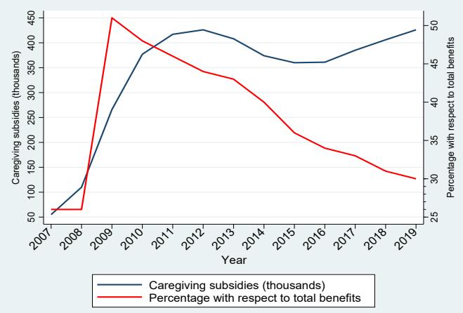
Although caregiving subsidies were originally intended in exceptional circumstances, they were granted in practice whenever no accredited public or private caregiver was available to deliver the required care in the ICP. Eligibility for a subsidy requires that the care be provided by a family member who has already been performing caregiving duties during the year preceding the application4. Figure 2 illustrates the trends in the total volume of caregiving subsidies over time, as well as their share relative to overall spending on SAAD subsidies and supports. The figure suggests that as the SAAD was rolled out, the uptake of caregiving subsidies declined as individual were able to find local caregivers alongside the specifications of the ICP.
Figure 1. Trends in long-term care spending in Spain
4 However, the monetary value of the subsidy covers only a small fraction of the actual cost of care and is further subject to co-payment deductions based on the beneficiary’s income level.
Note: This figure shows the evolution of long-term care spending as a percentage of GDP. The vertical line indicates the start of the SAAD. Source: OECD, 2023.
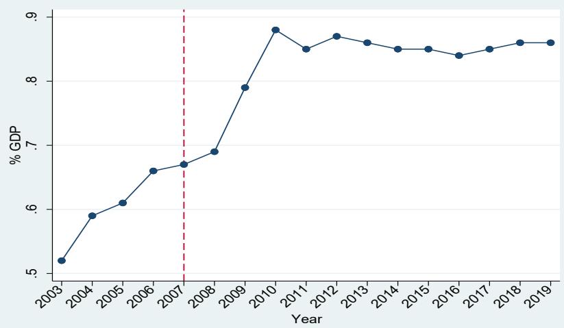
Figure 2. Caregiving subsidies as total caregiving subsidies (thousands) and % of total benefits Note: This figure shows the evolution of the number of caregiving subsidies: total number of people receiving this benefit and percentage of total benefits granted. Source: own work using data from Estadística mensual - Instituto de Mayores y Servicios Sociales (imserso.es)
Rollout of SAAD and austerity spending cuts. The rollout initially targeted individuals with severe (“major”) dependency in 2007 and was gradually extended to moderate levels of need. Table 1 reports the evolution of care hours and the monetary value of home-based support. However, following the European Commission’s recommendations, austerity measures led to an adjustment period between 2012 and mid-2015, slowing the expansion of the programme. Indeed, the Royal Decree 20/2012 of 13 July 2012 entailed a reduction of the benefits of SAAD to comply with public deficit targets and spending stagnated between 2011 and 2015 at around 0.7% of GDP (below the EU average of 1.6%) (European Commission, 2015).
[Insert Table 1 about here]
Co-payments were increased, requiring beneficiaries with monthly incomes above €532 - as of 2012- to contribute progressively more, up to 90% of service costs. This obligation, previously limited to residential care, which was subsequently extended to all services and cash benefits. These measures formed part of austerity adjustments following Spain’s 2012 public deficit (8.9%), leading to significant budget cuts to SAAD under Royal Decree 20/2012.
The measures introduced included a 13% reduction in the National Government’s contribution to financing the minimum level of protection, and the elimination of social security contributions for non-professional carers, which had previously been covered by the government—although carers could choose to remain in the scheme by paying the full amount themselves. Additionally, caregiving subsidies for informal caregivers were immediately reduced by 15%, alongside a cut in the hours provided by home help services. A maximum suspension period of two years was established for receiving caregiving subsidies from the date of eligibility. Altogether these measures represented an estimated budgetary saving of 2,278 million euros between 2012 and 2014.
The SAAD began to show signs of recovery in mid-2015, when there was an increase in the number of applications, the number of individuals assessed, and the proportion of SAAD beneficiaries relative to the total population, which contributed to a reduction in waiting lists (Jiménez-Martín and Viola, 2017). A key driver of this growth was the long-delayed incorporation of moderate dependents into the system, finally implemented from mid-2015. However, progress was hindered by additional financial constraints, particularly the failure to pass the general state budget bill for two consecutive years (2019 and 2020), resulting in continued reliance on the extended 2018 budget. A decade after the system's inception, the actual number of beneficiaries with entitlements had fallen significantly short of the projections. Nonetheless, in 2021 and 2022, the general state budgets included a substantial increase in longterm care funding—23.3% higher than in 2021 and double the amount allocated in 2018 (Jiménez-Martín and Viola, 2022).
4. Data and Empirical Strategy
4.1. Data and variables
Given the absence of a consolidated administrative dataset on long-term care services and supports in Spain, and the reliance on survey-based measures for health outcomes, we draw on the Spanish sample from SHARE (Survey of Health, Ageing and Retirement in Europe) for Wave 1 (2004), Wave 2 (2006/2007), Wave 4 (2011), Wave 5 (2013), Wave 6 (2015), Wave 7 (2017), Wave 9 (2021/2022).5 We do not include Wave 8 to avoid our estimates to be contaminated by the COVID-19 pandemic. SHARE is the European equivalent of the Health and Retirement Survey. SHARE interviews all individuals aged 50 and over at the time of sampling who have their regular residence in the respective SHARE country. All respondents who participated in any prior wave are included in the longitudinal sample. New partners residing in the household are also interviewed, regardless of age. Individuals are excluded from baseline or refreshment samples if they are institutionalised, abroad for the entire survey period, unable to speak the official language(s), or have an unknown address.
The Spanish SHARE sample follows the core survey design, ensuring representativeness across regions and key demographic characteristics, including age and gender. Previous studies have documented both the high quality and comparability of SHARE data across countries, as well as its suitability for population-representative analyses of individuals aged 50 and above. The Spanish SHARE sample is representative of the population aged 50+ living in private households, conditional on the use of appropriate sampling weights (Börsch-Supan et al., 2013; Bergmann et al., 2019).
5 Unfortunately, wave 3 could not be included as it is not comparable with the other waves.
The initial sample consists of 29,002 observations (2,711 for the pre-SAAD period (2004-2006) and 26,291 observations for the post-SAAD period (2007-2022). The sample is divided into three groups as depicted in Table 2, namely: (i) those receiving disability benefits or caregiving subsidies (4%-5%); (ii) individuals receiving home care supports (7% in the pre-SAAD period and 10% in the post-SAAD period); and (iii) individuals not receiving any type of subsidy or support (89%-86).
[Insert Table 2 about here]
We consider the following outcomes:
Life satisfaction. This (ordinal) variable is defined using the following question: ‘On a scale from 0 to 10 where 0 means completely dissatisfied and 10 means completely satisfied, how satisfied are you with your life?’.
Loneliness: Loneliness is a key risk factor for depression (Ge et al., 2017) and is associated with a range of adverse health outcomes, including dementia (Kuiper et al., 2015), suicidality (Stickley & Koyanagi, 2016), coronary heart disease (Valtorta et al., 2016), and increased mortality risk (Holt-Lunstad et al., 2015), contributing to higher healthcare expenditure (Mihalopoulos et al., 2019).
We use the short three-item version of the Revised UCLA Loneliness scale (henceforth, R-UCLA, Russell et al., 1978). The wording of the items is: “How often do you feel isolated from others? How often do you feel you lack companionship? How often do you feel left out?”. In each case, the available responses are: 1. Often, 2, Some of the time, 3. Hardly ever or never. SHARE has created a scale ranging from 3 (not lonely) to 9 (very lonely).
Depression. We use the EURO-D scale which has been applied to identify depressive symptoms in European countries (Prince et al., 1999). EURO-D is a 12-item scale in which the respondent is asked whether in the past month he/she has experienced any of the following symptoms: ‘depressed mood’, ‘pessimism’, ‘suicidality’, ‘guilty feelings’, ‘sleep problems’, ‘loss of interest’, ‘irritability’, ‘less appetite’, ‘fatigue’, ‘lower levels of concentration’, ‘less enjoyment in life’ and ‘tearfulness’. A score greater than 3 out of 12 signals a depressive disorder, for which therapeutic intervention would be recommended (Dewey and Prince, 2005).
Survival. Death is identified by linking the main questionnaire in one wave with the endof-life questionnaire in the subsequent wave. For deceased respondents, an end-of-life interview is conducted with a proxy, either in person or by telephone. Proxy respondents may include a family or household member, neighbour, or another close contact. This interview provides detailed information on the respondent’s final year of life and the circumstances surrounding death.. We define a binary variable that takes the value 1 if the individual has survived between two consecutive waves and 0 if the individual has died.
Since not all respondents from one wave participate in the next wave (due to unavailable localization), we investigated the potential presence of attrition bias. To do this, we estimated a series of attrition probit models following Fitzgerald et al. (1998) and conducted pooling tests to compare the equality of coefficients between the initial sample with and without attritors, using the Becketti-Gould-Lillard-Welch test (Becketti et al., 1988). Specifically, we first regressed the outcome variables from the first wave on household characteristics, an attrition indicator, and interactions between the attrition indicator and the explanatory variables. We then tested the joint significance of these interaction terms and the attrition indicator to assess whether the effects of the explanatory variables differ between households that attrite and those that remained in the sample. The results suggest that attrition is conditionally random, indicating it is unlikely to bias our estimates. The small pseudo-R-squared from the attrition probits, which can be interpreted as the proportion of the attrition that is not random, from the Becketti-Gould-Lillard-Welch test (Outes-Leon and Dercon, 2008), reinforces our previous diagnostic.
4.2.Empirical Strategy.
4.2.1. Coarsened exact matching
We examine whether the expansion of LTC access resulting from the introduction of SAAD exerted an impact on survival, depression, loneliness, and life satisfaction using a strategy that combines an innovative sample selection method, the coarsened exact matching (CEM), with either a Difference-in-Differences (DiD) or an event studies estimation strategy (plus other options for robustness). The introduction of SAAD enables a difference-in-differences design, comparing outcomes between recipients and nonrecipients of long-term care benefits before and after the programme’s rollout.
Our approach aims to ensure that treatment and control groups are as similar as possible in terms of covariate distribution (Ho et al, 2007), as well as between before and after introduction of the SAAD. The main advantage of the combination of DiD with CEM matching is that it ensures the robustness of our estimates in the sense that, under weak conditions, the causal estimates should be consistent (Ho et al., et al., 2007). The most widely used current methods, propensity score and Mahalanobis matching, belong to the class of matching methods known as 'same-percentage bias reducers', which do not guarantee any level of imbalance reduction in any given data set. Their properties hold only on average across all samples and even then, only by assuming several usually unverifiable assumptions about the data generation process. Iacus et al. (2011) show that CEM dominates existing commonly used matching methods in its ability to reduce imbalance, model dependence, estimation error, bias, variance, mean square error, and others. Furthermore, CEM works by sampling and requires no assumptions about the data generation process and guarantees that the imbalance between treated and matched control groups will be no greater than the user's ex ante choice.
CEM matching can be used with repeated cross-sectional data (Iacus et al. 2012, Heckman et al., 1998). The strategy consists of simultaneously matching using a set of possible confounders which are coarsened, reducing the number of possible matching values for a given covariate with the aim of increasing the number of matches achieved. The most widely used current methods, propensity score and Mahalanobis matching, belong to the class of matching methods known as 'same-percentage bias reducers', which do not guarantee any level of imbalance reduction in any given data set. Their properties hold only on average across all samples and even then, only by assuming several usually unverifiable assumptions about the data generation process. Iacus et al. (2011) show that CEM dominates existing commonly used matching methods in its ability to reduce imbalance, model dependence, estimation error, bias, variance, mean square error, and others.
Unlike propensity score matching (PSM), which requires model estimation and iterative ex-post balance checking, CEM applies exact matching on temporarily coarsened covariates, guaranteeing that adjustments to imbalance on one dimension do not inadvertently worsen imbalance on others (Iacus et al. 2012). This design-based approach yields matched samples with bounded imbalance, reduced model dependence, and automatic restriction to common support, thereby preventing the extrapolation problems frequently observed with propensityscore-based pruning. Because CEM is nonparametric, transparent, and extremely fast, it facilitates a preprocessing stage that approximates a blocked experimental design, on which subsequent outcome models can be estimated with markedly lower risk of misspecification.
In contrast, a substantial body of methodological research shows that PSM can increase imbalance, inefficiency, and bias under common applications. Specifically, PSM approximates a completely randomized experiment rather than a blocked design, making it “blind” to sources of imbalance that other matching methods, including CEM, can eliminate (King & Nielsen, 2019). When pruning becomes aggressive (e.g., tightening calipers), PSM may even produce more imbalance than the original data, a phenomenon known as the PSM paradox (King & Nielsen, 2019). Although comparative studies confirm that CEM may lose precision when applied to very high-dimensional covariate sets, they also show that CEM generally achieves superior multivariate balance, especially when the analyst can identify a focused set of strong confounders and define substantively meaningful coarsenings (Ripollone et al., 2020). Tetteh et al. (2019) have found that CEM is preferable to other matching procedures (e.g. propensity score matching) in terms of more efficient processing and reduced model dependence, variance and bias.Given these properties, CEM provides a more robust and defensible design stage for our study, ensuring that subsequent causal estimates rest on tightly controlled imbalance and reduced reliance on outcome-model assumptions.
Our choice is based in the fact that CEM reduces any imbalance in covariates between treated and control units. CEM incorporates properties of the exact matching procedures and allows the balance between treated and control groups to be chosen ex-ante. After applying the CEM method, a weighting variable is retrieved to equalise the number of observations within the comparison groups.
We define for each year (before and after the introduction of SAAD), two groups of respondents of SHARE, selecting age, gender, marital status, years of education, income, and comorbidities as pre-treatment covariates for matching because the literature on long-term care (LTC) consistently shows that these factors jointly shape both need for care and assignment to care modality (formal home care vs. informal/family care), as well as access and intensity of SAAD benefits.
Age. LTC need and intensity rise sharply with age, with steep increases in ADL/IADL limitations among the 80+ population. In Spain, demographic aging and the high share of oldest-old are central drivers of LTC use, including home care and allowances (Costa-Font et al., 2023; WHO/WKC Spain case study). Matching on age thus helps balance baseline need and the probability of qualifying for, and substituting between, formal services and cash-for-care.
Gender. The Spanish system exhibits pronounced gender asymmetries: women are both more likely to need care (given longevity) and overwhelmingly more likely to provide it (informal and formal). Evidence for Spain documents that women account for most caregivers in both spheres, influencing the chances that a dependent person receives family care versus contracted services (Costa-Font et al., 2023a; WHO country brief). Controlling for gender addresses systematic differences in care availability and modality.
Marital status. Spousal availability is a strong predictor of informal care receipt; countries and reports emphasizing support to informal carers routinely list identification and inclusion of family carers as a key determinant of care arrangements (Eurocarers policy briefing; WHO country brief for Spain). In Spain’s SAAD, the presence of a spouse/partner often shifts the margin between formal home help and allowances linked to informal care.
Years of education. Education proxies health literacy, navigation capacity, and social capital, which affect application, take-up, and the mix of services vs. allowances chosen within SAAD’s menu (WHO/WKC case and country brief; Díaz-Tendero & Ruano, 2024). Higher education tends to correlate with more successful access to formal services, and with preferences for professional care rather than demanding family care regimes.
Income. In Spain, SAAD includes co-payments and income-/wealth-sensitive contributions; affordability constraints and the distribution of cash benefits vs. in-kind services vary across regions and income levels (WHO/WKC Spain; WHO country brief). Consequently, income influences both eligibility to specific options and care modality, making it a key confounder for formal home-care receipt. Broader EU evidence also links underfunding and user charges to substitution away from formal services toward informal care (European Commission, 2021).
Comorbidities (health status/functional need). Eligibility and intensity in SAAD are graded by dependency severity (functional limitations and health status). Comorbidities raise care intensity and tilt choices between home help, day centers, residential care, and cash for informal care; Spain’s reports repeatedly emphasize that degrees of dependency channel beneficiaries to different service portfolios (WHO/WKC Spain; WHO country brief).
In short, these six covariates jointly capture need (age, comorbidities), household supply of caregiving (marital status, gender), and socioeconomic/behavioural capacity to access and finance care (education, income)—all of which are theoretically and empirically linked to care modality under SAAD.
An additional advantage of the CEM estimator over the standard matching procedure is that it allows us to control for unobserved time invariant factors. This implies that we assume that the outcome variables of interest of the treated and control units, in the absence of any treatment show the same growth trajectory, i.e., the parallel trend assumption of the DiD method.
Table B2 documents comparable descriptive statistics for socio-demographic variables for the initial sample and the sample after CEM. Table B3 also compares the L1-statistic the initial sample (29,002 observations) and the sample obtained after applying CEM (26,738). In Coarsened Exact Matching (CEM), the L1 statistic is a multivariate imbalance measure computed over the joint histogram of coarsened covariates that quantifies how dissimilar the treated and control distributions are after coarsening; it is effectively a normalized total variation (Manhattan) distance between the two empirical distributions across strata defined by the chosen bins, where L1 = 0 indicates perfect global balance and larger values indicate worse balance (and less overlap) (Iacus et al., 2012). Practically, analysts report pre-match vs. post-match L1, using the reduction in L1 as an aggregate indicator that the design stage improved balance beyond univariate checks; because L1 is computed on the joint distribution, it can reveal imbalances invisible to single-covariate diagnostics. We appreciate a significant reduction in imbalance for all explanatory variables.
4.2.2. Event Study.
We estimate the following event-study specification:
\[Y _ {i r t} = \sum_ {j \neq - 1} \beta_ {j} 1 \{\rho_ {i t} = j \} + X _ {i r t} ^ {\prime} \alpha_ {1} + E _ {t} + R _ {r} + T _ {t} + \varepsilon_ {i r t}\tag{1}\]
where is the outcome variable (depression, life satisfaction, loneliness and survival) of individual i living in region r and interviewed in year t. denotes the leads and lags of SAAD implementation, which allow us to analyze non-parametrically differences between beneficiaries and non-beneficiaries of SAAD in years prior to and after the onset of SAAD.
refers to a vector of control variables including the respondent’s sociodemographic characteristics (age, sex, marital status, level of education, body mass index, degree of dependency rated by the Katz’s index6, self-reported health status, chronic illness, smoking and drinking habits, days stayed at hospital during last year for surgery or medical tests, days stayed at hospital during last year due to mental health problems, number of days stayed in other institutions other than a hospital or a nursing home during last year (i.e., institutions for rehabilitation, convalescence), visits to general practitioner during last year, sedentary lifestyle, living alone, living in a rural area).
6 The Katz Index (Katz, 1983) determines functional status as a measurement of the ability to perform six ADLs independently. We have computed this index using the information on ADLs provided by SHARE. Respondents have been classified into four categories: Katz_0 indicates that the individual performs all activities independently; Katz_1 indicates that the individua performs four or five activities independently; Katz_2 indicates that the individual only performs two or three activities; Katz_3 indicates that the individual needs help for all these activities (or all but one)
is a vector of regional economic characteristics according to the respondent’s place of residence (real per capita GDP, unemployment rate), which helps to control for the effect of potentially relevant macroeconomic conditions. All regressions are estimated using calibrated sampling weights.7 Finally, and denote regional and year fixed effects, respectively, and is an individual-specific error term.
Evidence that beneficiaries and non-beneficiaries exhibit similar time-varying changes in outcomes prior to SAAD is suggestive of the presence of parallel trends. Furthermore, we directly test whether beneficiaries and non-beneficiaries present different pre-reform trends by means of a joint F-test that all pre-SAAD dummies are equal to zero
4.2.3. Difference-in-differences
Several studies have used a DiD strategy to analyse the effect of the introduction of a new policy (Winkelmann, 2004; Chou et al., 2010). Our empirical strategy relies on a DiD design with staggered treatment adoption (Callaway and Sant’Anna, 2021), where treatment status is absorbing. In this model estimation, we consider the overall effect of the SAAD; that is, we distinguish between the pre-SAAD period (2004–2006) and the post-SAAD period (2007–2020). Subsequently, in Section 7, we have included an extension to estimate the effect of the budgetary cutbacks (2012–2017).
The treated group consists of individuals who receive long-term care benefits in Spain after the implementation of the SAAD reform, either in the form of caregiving subsidies or home care assistance . The control group is defined as individuals who do not receive any type of long-term care support (neither cash benefits nor in-kind home care services) throughout the observation period. The main comparison of interest is therefore between individuals who transition into SAAD benefits after the reform and those who were either untreated or received different types of support prior to the reform, thus capturing the differential effect of the SAAD policy relative to the pre-existing system. Specifically, we compare changes in outcomes for individuals who receive long-term care benefits under the SAAD system after its implementation with the counterfactual evolution of outcomes among individuals who do not receive any form of LTC support. In addition, we exploit the institutional shift from pre-SAAD benefits —such as disability allowances and home care benefits — to post-reform benefits —caregiving subsidies and home care assistance — in order to identify the incremental effect of the reform. This approach allows us to distinguish between the effect of receiving LTC support per se and the additional effect attributable to the SAAD reform.
7 SHARE provides two types of weights. The sampling design weights are defined as the inverse of the probability of being included in the sample of any specific wave. Although these weights compensate for the unequal selection probabilities of the sample units, unbiased estimators of the population parameters can only be obtained under the ideal situation of complete response. Unfortunately, given that SHARE data are affected by problems of unit non-response and sample attrition, estimators constructed using sample design weights alone may be biased (Lessler and Kalsbeek, 1992). The strategy used by SHARE to cope with these problems relies on the ex-post calibration procedure of Deville and Särndal (1992).
Our specification is defined as follows:
\[Y _ {i r t} = X _ {i r t} ^ {\prime} \alpha_ {0} + \alpha_ {1} E _ {r t} + \alpha_ {2} D A _ {i r t} + \alpha_ {3} C _ {i r t} + \alpha_ {4} H C B _ {i r t} + \alpha_ {5} H C A _ {i r t} + R _ {r} + T _ {t} + \varepsilon_ {i r t}\tag{2}\]
is the outcome (loneliness, life satisfaction, depression symptoms, survival probability8) of respondent i living in region r in year t. The key covariates of our specification are as follows: (i) is a binary variable equal to 1 if the care recipient received a disability allowance before the SAAD, and 0 otherwise; (ii) is a binary variable equal to 1 if the care recipient received an allowance from the SAAD, and 0 otherwise; (iii) homecare support , is a binary variable equal to 1 if the care recipient received publicly funded homecare before the SAAD, and 0 otherwise; and (iv) is a binary variable equal to 1 if the care recipient received publicly funded homecare support after the SAAD, and 0 otherwise.
The linear probability model turns out to be a much more friendly environment, as compared to a probit model, for detecting and interpreting the coefficients of interaction terms (Angrist & Pischke, 2009). Ai and Norton (2003) show that the interaction effect in a nonlinear probit model is not necessarily equal to the marginal effect in the linear probability model. In non-linear models the ordinarily reported standard errors and marginal effects of interacted variables require corrections. For the benchmark specification we compare the standard errors of the linear probability model, with the non-corrected and corrected standard errors of the probit model
as in equation (1), refers to a vector of control variables including the respondent’s sociodemographic characteristics,9 is a vector of regional economic characteristics according to the respondent’s place of residence (real per capita GDP, unemployment rate), which helps to control for the effect of potentially relevant macroeconomic conditions; and denote regional fixed effects and year fixed effects, respectively, and is an individualspecific error term.
We have addressed potential endogeneity concerns by estimating an instrumental variable model as in Costa-Font et al. (2022)10. All instruments used were relevant, and do not reveal weak instrument concerns as they are all decision taken before the reform and exerted no influence on it. IV and OLS estimates, including 95% confidence intervals, were highly consistent. However, as discussed in Bertrand et al. (2004), one of the concerns is that the difference-in-difference specifications may underestimate the standard errors coefficient. We overcome this problem by applying block bootstrap (Efron and Tibshirani, 1994), because it maintains the autocorrelation structure, grouping all the observations that belong to the same region.
Given the progressive implementation of SAAD, treated individuals are those classified as highly dependent in 2007, while SAAD in 2011 included the latter, those classified as severe, and some moderate dependents (Level 2). Finally, from onwards, SAAD covered all dependents. Our main coefficients of interest are and which measure the effect of caregiving subsidies and home supports after the SAAD on the four outcomes of interest.
9 We categorize the explanatory variables in several groups (see Table B1 for the precise definition of these variables and Table B2 for descriptive statistics): (i) demographic characteristics (age, sex, marital status, and level of education); (ii) health and lifestyle variables (body mass index, degree of dependency rated by the Katz's index, chronic illness, smoking and drinking habits, self-reported health status and sedentary lifestyle; (iii) use of healthcare services (days stayed at hospital during last year for surgery or medical tests, days stayed at hospital during last year due to mental health problems, number of days stayed in other institutions other than a hospital or a nursing home during last year (i.e., institutions for rehabilitation, convalescence), visits to general practitioner during last year); (iv) household and environmental related variables (living alone, living in a rura area, adjusted income and wealth)
10 The instruments include whether the socialist party runs the regional government - given that it was a proposal of the socialist party in power and hence its electoral commitment to the implementations of the LTC reform: the 2004 publicly funded homecare coverage index, the 2004 average monthly homecare hours and the 2004 public cost per hour. These variables capture pre-SAAD regional variations in formal care provision which could have influenced the speed of the reform.
4.2.4. Specification checks.
A plausible identification problem is that the awarding of LTC benefits may be correlated with other contemporary shocks. For example, the incidence of the economic crisis in 2008 may have difficulted the rollout of the SAAD. To address this concern we include the unemployment rate in the vector of controls. Second, we run a falsification test based on the change in unemployment rate between 2008 and 2013. We bin regions in 4 quartiles and reestimate equation (2) with quartile-by-year fixed effects. This specification allows us to test that common time shocks across regions varying according to recession severity have no effect on our results.
We also check if the relationship between the outcomes of interest and the SAAD benefits arises from unobserved common shocks. For example, increasing life expectancy could lead to a spurious correlation between the outcomes and the SAAD resulting from the overarching trends, but not by the LTC policy itself. To address this concern, we consider additional specifications that include common shocks using region-specific linear trends and a fixed effects model with interactions.
A common concern in difference-in-differences settings is that treated and control units may follow different underlying trends. To account for this possibility, we augment (2) with region-specific linear time trends:
\[Y _ {i r t} = X _ {i r t} ^ {\prime} \alpha_ {0} + E _ {r t} ^ {\prime} \alpha_ {1} + \alpha_ {2} D A _ {i r t} + \alpha_ {3} C _ {i r t} + \alpha_ {4} H C B _ {i r t} + \alpha_ {5} H C A _ {i r t} + R _ {r} + \gamma_ {r} t + \varepsilon_ {i r t}.\tag{3}\]
11 However, health-related variables recorded in SHARE do not allow distinguishing between the three degrees of dependency because the ranking scale used by SAAD involves a higher number of ADLs.
This specification absorbs gradual, region-specific evolutions that could otherwise confound policy effects, while still leveraging within-region variation over time.
Linear trends may be too restrictive if regions respond differently to aggregate shocks in a non-linear manner. We therefore estimate a more flexible model with interactive fixed effects, which allows for non-linear region-specific time patterns generated by a small number of unobserved common factors:
\[Y _ {i r t} = X _ {i r t} ^ {\prime} \alpha_ {0} + E _ {r t} ^ {\prime} \alpha_ {1} + \alpha_ {2} D A _ {i r t} + \alpha_ {3} C _ {i r t} + \alpha_ {4} H C B _ {i r t} + \alpha_ {5} H C A _ {i r t} + R _ {r} + f _ {t} ^ {\prime} \lambda_ {r} + u _ {i r t}.\tag{4}\]
In (4), is a vector of time-varying common factors and is a vector of regionspecific factor loadings. This low-rank component �captures unobserved common shocks (e.g., macroeconomic, institutional, or health-system shocks) that affect all regions but with heterogeneous intensity, thereby accommodating potentially non-linear region-specific trajectories over time, and an idiosyncratic component. This approach follows the interactive effects (linear factor) framework discussed by Gobillon and Magnac (2016).
5. Results
5.1. Event study estimates.
Figure 3 presents the main results. With only two pre-treatment observations, the parallel trends assumption appears to hold for three of the four outcomes, though this may raise concerns about robustness. To address this, we exploit semi-annual variation in the data to increase the number of pre-treatment periods. Figure A5 in the Appendix replicates the analysis with two additional pre-treatment observations, showing that the parallel trends assumption is satisfied across all outcomes under this specification.
Figure 3. Event-study of the effect of access to long term care servicies and supports on health and wellbeing
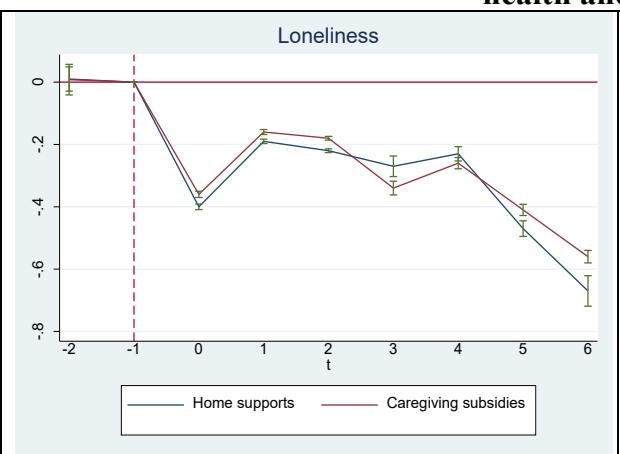
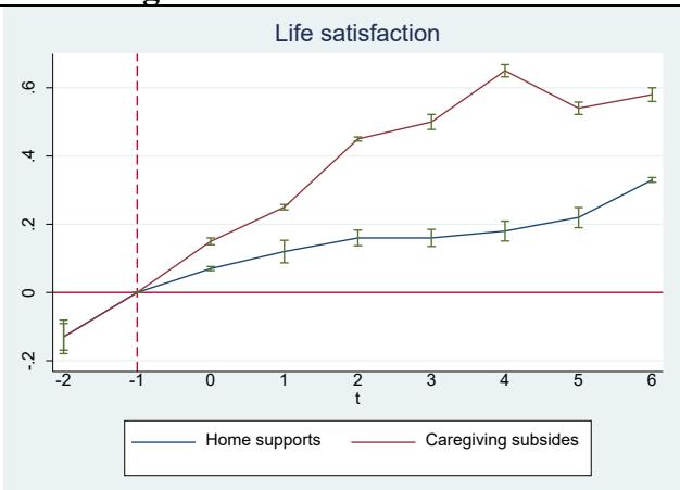
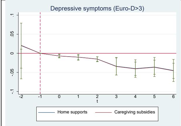
Note: This table displays the event study coefficients of the four outcomes of interest for individuals receiving care subsidies and home care supports. Period 0: implementation of SAAD. Period -1 corresponds to pre-SAAD situation (year 2004). Periods 1 to 6 corresponds to the situation after SAAD. Source: Own work using SHARE.
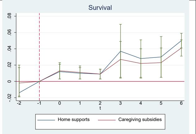
Turning to policy effects, we find significant changes in three outcomes following the introduction of SAAD: higher life satisfaction and survival probability, and lower loneliness. The effects on survival and loneliness are significant and of similar magnitude across both caregiving subsidies and home care support programmes. In contrast, the increase in life satisfaction is substantially larger among home care recipients. The estimated effect on depression is negative, but not statistically significant.
Given the short pre-reform window, standard pre-trend tests have limited power and conditioning on their insignificance may bias inference (Roth, 2022). We therefore do not rely solely on these tests, and instead complement the event-study analysis with robustness and sensitivity checks. In particular, we implement an Honest DiD approach (Rambachan and Roth, 2023), which bounds potential post-treatment deviations from parallel trends relative to observed pre-treatment differences..
Specifically, we compare the size of deviations in the pre-SAAD period with effects observed after SAAD; if post-SAAD effects are larger, this supports the presence of a genuine treatment effect. To operationalize this, we compute adjusted confidence intervals based on multiples (0.1, 0.25, 0.5, 1, and 2) of the largest pre-treatment deviation and contrast them with the original 95% confidence interval that assumes no trend violation. As illustrated in Figure A6, our estimates remain robust even when allowing for violations up to twice the magnitude of the largest pre-SAAD difference, meaning the effects persist under sizable relaxations of the parallel-trends assumption. Hence, reversing our baseline estimates would require post-treatment departures substantially larger than anything observed prior to treatment.
5.2. DiD estimates.
Table 3 displays our main estimates for the four main outcomes—loneliness, life satisfaction, depressive symptoms, and survival—based on the CEM-corrected sample and a pooled OLS DiD model, across four progressively nested specifications using the yearly data. In the next comments, we focus on the specification which includes the most complete set of explanatory variables (M4).
Post-SAAD reduces loneliness in 0.61 points for caregiving subsidies and 0.52 points for home care supports. While disability allowances had a significant pre-reform effect of – 0.52 points, home care supports showed no significant pre-reform impact. This indicates that the “protective” effect against loneliness has increased by 18% for caregiving subsidies, and that home care supports now significantly reduce loneliness—although by 15% less than subsidies. Life satisfaction rises by 0.24 Likert points among those receiving subsidies and 0.50 Likert points among those with home care supports post-reform, with no pre-reform benefits showing significant effects; the impact of home care supports is twice that of subsidies in this case.
Exposure to SAAD reduces depressive symptoms by 1 pp for caregiving subsidies and 0.8 pp for home care supports, with no pre-reform effects and a 13% stronger impact for subsidies. After the reform, survival rises by 3 pp and 2.6 pp, respectively, again with no pre-SAAD differences. Overall, the estimates indicate that SAAD improves all outcomes: subsidies are more effective in reducing loneliness and depression and in increasing survival, while home care support yields larger gains in life satisfaction, consistent with its stronger association with longevity.
[Insert Table 3 about here]
5.3.Specification exercises.
To enhance the reliability of the estimates in Table 3, we have carried out some additional analyses. First, by introducing half-yearly time fixed effects instead of yearly time fixed effects. Figure A7 shows a comparison with the estimates in Table 3 (M4), suggesting barely any difference in the magnitudes of the coefficients.Second, Table C1 presents the estimates corresponding to specification (3), which includes a region-specific linear trend, and Table C2 shows the estimates including time-varying common factors with heterogeneous effects across cross-sections, respectively.
Finally, to facilitate a better comparison of these alternative specifications, Figure C1 compares our main estimation (Table 3; M4) with Equation 3 (an alternative specification incorporating region-specific linear trends and a fixed-effects model with interactions),
Equation 4 (an alternative specification with a multi-factor structure of time-varying common factors with heterogeneous effects across cross-sections) and a falsification test (dividing the regions into four quartiles according to the 2008–2013 unemployment rate and re-estimating with quartile-by-year fixed effects). We observe that the sign and significance of the coefficients are maintained, but those of the alternative specifications show larger effects (in absolute terms). Therefore, the main specification (Table 3: M4) can be considered as a lower (conservative) threshold for the long-term effects of the SAAD on outcomes.
5.4.Heterogeneity.
This section examines heterogeneous effects of caregiving subsidies and home care support across four outcomes. We consider heterogeneous effects by age, sex, place of residence, household size, dependency level, income, and wealth. Tables A1–A4 report OLS-DiD estimates based on the CEM-adjusted sample.
Gender. The impact of home care supports on loneliness is 133% higher for women (- 0.58 points versus -0.44 points) and the impact on the probability of survival is very small for men (only 1.3pp for home care supports), but much more significant for women (4.6pp for caregiving subsidies and 3.6pp for home care supports).
Age. The reduction in loneliness derived from receiving home care supports is increasing with age (from -0.20 points for 50-64 years to -0.47 points for 80 years and older). The greatest increase in the probability of survival corresponds to the cohort aged 80+ receiving caregiving subsidies (+5.6 pp.), twice as much as when receiving home care supports (2.8 pp.) in the same age cohort, and four times more than for the 65-79 cohort (1.2pp-1.3pp.).
Place of residence. For all outcomes, receiving caregiving subsidies or home care supports results in a decrease in loneliness and depression or an increase in life satisfaction and survival that is more intense for people living in a rural area. Receiving caregiving subsidies increases life satisfaction (0.95 points in rural areas and 0.27 points in urban areas), which is a beneficial effect in both cases, but 353% more intense in rural areas.
Household size. Receiving some type of LTC benefit has a stronger positive or negative impact for people living alone. And in the case of living alone, the effect is stronger for caregiving subsidies. Although this benefit is designed to be awarded to co-residents caregivers, in exceptional situations (for example, living in an isolated environment) it can also be provided by non-co-resident family members or neighbours. It is noteworthy that, in this case, the indicator of loneliness decreases by 0.76 points, while that of satisfaction with life increases by 1.16 points.
Care needs. Approximating the level of dependency using the Katz index (moderate: 1, 2; severe; 3,4; highly dependent; 5, 6), we have estimated the impact of LTC benefits on the four outcomes. Receiving caregiving subsidies (home care supports) has decreased loneliness and depression in both groups of dependents, but the effect has been greater for severe dependents (it has decreased 107% (92%) for loneliness and 128% (156%) for depression). The increase in the probability of survival for highly dependent (2.7pp. for both benefits) is very encouraging, although this effect is 43% (52%) higher for the severely dependent (depending on whether caregiving subsidies were received, 6.3pp or home care supports, 5.2pp).
6. Mechanisms
Next, we the literature identifies four potential mechanisms as follows: (i) nutrition; (ii) maximal grip strength; (iii) locus of control; and (iv) hip or other bones fractures.
Nutrition. Access to regular care from an informal or formal caregiver may result in improved diet and reduced risk of malnutrition. For each of the following food categories "dairy products", "legumes, beans or eggs" "fruits or vegetables" and "meat, fish or poultry" we defined a binary variable that takes the value 1 if they are consumed at the indicated frequency: "every day", "3-6 times a week", "twice a week", "once a week" or "less than once a week", and 0 otherwise. These food groups respond literally to the SHARE questions, and it is not possible to know the frequency of consumption of "legumes" and "eggs" separately, or of "meat" and "fish" separately.
Maximum grip strength. Hand grip strength has a significant inverse association with depression (Brooks et al., 2018), and is a long-term predictor of all-cause mortality, cardiovascular disease, and cancer in men (Gale et al., 2007). Higher prehensile strength is associated with better quality of life overall, as well as in the domains of autonomy, satisfaction with past, present, and future activities and achievements, and satisfaction with social participation (Xie and Ma, 2021). We have defined a continuous variable that collects the respondent's maximum handgrip strength with the aid of a dynamometer.
Locus of control. This variable reflects "whether or not the person perceives a causal relationship between his or her own behaviour and reward" (Rotter, 1966), and may be differentiated between “internal locus of control” when people believe that they control life outcomes and their own destiny, versus “external locus of control” when they believe that what happens in life is mainly due to external factors, such as fate, luck, or other people. Wong and Anitescu (2017) show that patients with an internal locus of control are less depressed than patients with a fatalistic view of their health/pain. We have measured locus of control through the question "How often do you feel that what happens to you is out of your control?" and defined four binary variables corresponding to the possible answers, which take the value 1 if the individual stated "often", "sometimes", "rarely" or "never", and 0 otherwise.
Fractures. Mortality and ill health resulting from fractures are the result of nutritional deficiencies. Karpouzos et al. (2017) show that insufficient intake of certain vitamins, especially A and D, and other nutrients, such as calcium, can affect bone health or even the time and degree of bone healing in the event of a fracture. Lonely older adults are more likely to suffer falls in the future (Zeytinoglu et al., 2021). Depression may also be the cause of fractures, influenced by medication and dysregulated biological and lifestyle factors in depression (Wu et al., 2010).
Nutrition. Table 4 reports OLS-DiD estimates of nutrition outcomes using the CEM sample. Prior to SAAD, disability allowances and home care support show no significant effects. Following implementation, beneficiaries exhibit significant dietary improvements: daily dairy consumption increases by 3.6pp (1.2pp), fruit and vegetable intake by 2.8pp (2.5pp), daily meat/fish/poultry consumption by 4pp (7.9pp) or 3–6 times weekly by 3.3pp (3.7pp), and legume/bean/egg consumption (3–6 times weekly) by 6pp (4.2pp).
[Insert Table 4 about here]
Maximum grip strength. Table 5 presents OLS-DiD estimates of maximum grip strength using the CEM sample. Individuals receiving LTC allowances, before or after SAAD, show lower grip strength; however, this gap narrows post-SAAD—from −4.92 kg (−2.93 kg) for men (women) with disability allowances to −1.98 kg (−2.41 kg) with caregiving subsidies, and from −6.42 kg (−3.73 kg) to −4.36 kg (−1.95 kg) for home care supports. The improvement is particularly pronounced among those aged 80+, with increases of 4.23 kg (1.63 kg) for men (women) with caregiving subsidies and 3.2 kg (1.9 kg) with home care supports.
[Insert Table 5 about here]
Locus of control. Table 6 reports OLS-DiD estimates of locus of control using the CEM sample. Before SAAD, the likelihood of perceiving things as “out of control” rose by 0.23pp (0.37pp) for men (women) with disability allowances and by 47.8pp (40.9pp) for those with home care supports. Post-SAAD, the pattern reverses: the probability of believing that things are “never out of control” increases by 11.8pp (14.1pp) for men (women) with caregiving subsidies and by 16.1pp (13.5pp) for home care support recipients.
[Insert Table 6 about here]
Fractures. Table 7 presents OLS-DiD estimates of fracture probabilities using the CEM sample. Before SAAD, no significant effects are observed. After implementation: (i) caregiving subsidies reduce hip (other) fractures by 2.4pp (1.6pp) for men and 7.1pp (3.6pp) for women; (ii) home care supports reduce them by 2.1pp (4.6pp) for men and 6.9pp (3.6pp) for women; (iii) effects are concentrated among men aged 65–79 and women aged 50–79; and (iv) among women, home care supports reduce hip fractures by 15.7pp (12pp) in these cohorts.
[Insert Table 7 about here]
7. Extensions
7.1.Effect of COVID-19 pandemic (Wave 8)
Wave 8 of the Survey of Health, Ageing and Retirement in Europe (SHARE) was unique primarily due to its drastic methodological adaptation in response to the COVID-19 pandemic. Fieldwork, which began in October 2019, was interrupted in March 2020, forcing a switch from face-to-face interviews to telephone surveys. The data collection included both the prepandemic CAPI interviews (Oct 2019–March 2020) and the subsequent CATI "Corona" interviews. The pandemic disrupted the scheduled "refreshment sample" (recruitment of new participants). Despite the forced interruption, the survey maintained high panel stability, with many respondents participating in the telephone-based COVID-19 survey (Bergmann and Börsch-Supan, 2021).
During COVID-19, restrictions aimed at protecting older adults reduced in-person contact and disrupted support networks, contributing to higher loneliness and mental health risks (Berg-Weger & Morley, 2020; Kadowaki & Wister, 2022). LTC benefits may mitigate these effects by sustaining assistance with daily activities and preserving routine and contact, thereby reducing the “support gap” created by lockdowns and reduced informal care (OECD, n.d.; Office of the U.S. Surgeon General, 2023). Pandemic evidence shows that loneliness is strongly associated with lower life satisfaction, supporting the view that policies preserving support and assistance can improve subjective wellbeing. For instance, cross-sectional evidence finds that loneliness explains substantial variation in mental wellbeing and life satisfaction, with higher loneliness and lower life satisfaction during COVID-19 (Lorber et al., 2023). Similarly, integrative reviews document widespread increases in loneliness and declines in quality of life during the pandemic (Bissett et al., 2026). Consistent with this, LTC benefits that sustained support during COVID-19 may have raised life satisfaction by mitigating isolation and maintaining daily functioning and perceived security (Lorber et al., 2023; OECD, n.d.).
Although the survival channel is nuanced, the link between social connection, mental health, and mortality is well established, providing a basis for testing the effects of sustained care and support on survival. The U.S. Surgeon General’s Advisory highlights associations between social connection, mortality, and mental health outcomes (Office of the U.S. Surgeon General, 2023). At the same time, LTC settings faced substantial COVID-19 risks: evidence documents high infection and mortality rates in facilities, alongside reduced transmission following restrictions on visits and group activities (Zhang et al., 2023). This suggests that community-based LTC benefits, by enabling safer care arrangements and continuity of support, may have improved outcomes—including survival—by limiting both infection risk and severe social isolation (Office of the U.S. Surgeon General, 2023; Zhang et al., 2023).
A key contribution is distinguishing between caregiving subsidies and home care support, which operate through different mechanisms, especially during COVID-19. Caregiving subsidies provide flexibility to substitute disrupted formal care with informal or privately arranged care, helping avoid unmet needs and sustaining social ties, thereby reducing loneliness and depression (Curl & Roberts, 2023; Lorber et al., 2023).In contrast, home care support delivers professional assistance and regular contact, which can directly reduce isolation, particularly for those living alone. However, its effectiveness during the pandemic depended on service continuity, which was sometimes constrained by disruptions and infection-control measures (OECD, n.d.).
Table C3 reports estimates for equation (2) including Wave 8 (CEM sample; +2,240 observations). Results remain consistent across specifications, with stronger post-reform effects. Caregiving subsidies (home support) reduce loneliness by 6.12% (5.19%) and depression by 10.10% (8.70%), while increasing life satisfaction by 4.80% (10.02%). Survival gains are largest, rising by 24% and 20.80%, respectively.
Overall, LTC benefits improve all outcomes, though effects differ by programme. Home support has a stronger impact on life satisfaction, while caregiving subsidies more strongly enhance survival and reduce depression. These differences reflect underlying mechanisms: home support provides direct assistance and social contact, whereas subsidies enable flexible care arrangements that help maintain continuity of care during disruptions such as COVID-19.
7.2.Effect of budgetary cutbacks (2012-2017).
Reduced public support increases unmet care needs, raising risks of health deterioration. It also exacerbates social isolation and loneliness, which are strongly associated with depression, lower life satisfaction, and higher mortality (Office of the U.S. Surgeon General, 2023; Berg-Weger & Morley, 2020). In parallel, greater reliance on informal care can intensify caregiver burden, generating additional negative effects for both caregivers and recipients (Gagliardi et al., 2022).
Empirical evidence supports these mechanisms. In England, reductions in social care spending are associated with higher old-age mortality (Loopstra et al., 2016), while increased spending reduces mortality and post-2010 constraints are linked to excess deaths (Martin et al., 2021; Watkins et al., 2017). Spending cuts are also associated with worsening health and quality of life (Stokes et al., 2022). Evidence from the Netherlands further shows that tighter eligibility and shifts towards informal care can reduce perceived care sufficiency and create adjustment costs (van Ginneken & Kroneman, 2015; Gardeniers, 2025).
Table C4 confirms these patterns. Austerity-driven cuts between 2012 and 2017 significantly offset SAAD’s benefits, increasing loneliness and depression while reducing life satisfaction and survival. Counterfactual estimates suggest that, without these cuts, improvements would have been substantially larger, particularly for survival.These findings highlight the welfare and mortality costs of LTC retrenchment and underscore the importance of protecting LTC programmes from pro-cyclical cuts during economic downturns.
8. The QALYs and Cost per QALY estimation
This section presents a detailed estimate of the cost per QALY using quality-of-life evidence from the data. Health-related quality of life is measured with the EQ-5D-5L instrument, while a composite outcome index is constructed to capture key long-term care outcomes, including life satisfaction, depression, loneliness, and survival. A generalized least squares model with a log-link Gaussian specification is then used to estimate health-related quality-of-life decrements, incorporating interactions between the previous outcome index and different types of benefits. Finally, the study calculates the monetary costs of long-term care benefits and models their relationship with health-related quality of life to assess costeffectiveness.
Cost-effectiveness is evaluated by comparing incremental costs with established thresholds for the maximum acceptable cost per QALY gained in public long-term care systems. Across Europe, these thresholds typically range between €20,000 and €50,000 per QALY, although they vary by country and policy context. For example, the UK’s NICE commonly applies thresholds between €23,000 and €35,000 per QALY, while countries such as the Netherlands and Sweden use broader ranges linked to disease severity or societal impact. Norway may accept thresholds as high as €120,000 per QALY for severe conditions, whereas Germany applies incremental cost-effectiveness analysis informally despite lacking an official threshold. Full methodological details and calculations are provided in Appendix D.
Table 8 reports the estimated coefficients from the QALY analysis, including years and days of life gained and the associated cost per QALY. The analysis examines the effects of caregiving subsidies and home care support costs, both expressed in annual logarithmic euro values so that coefficients can be interpreted as elasticities. Results show that a 1% increase in caregiving subsidies or home care support expenditure is associated with increases of 0.00087% and 0.00053% in average QALYs, respectively.
Evaluated at the average expenditure level by sex and age cohort, an additional €1 per beneficiary per year increases QALYs by 0.0029 for caregiving subsidies and 0.0020 for home care supports. Expressed in days, these gains correspond to 1.09 additional days for caregiving subsidies and 0.73 days for home care supports. Using an average life expectancy of 18.4 years for the relevant population group, the estimated cost per QALY is €6,187.45 for caregiving subsidies (€5,815.96 for men and €6,398.95 for women) and €9,227.61 for home care supports (€7,498.42 for men and €10,553.20 for women). These estimates are substantially below commonly applied European cost-effectiveness thresholds, suggesting that both interventions provide good value for money in long-term care systems.
[Insert Table 8 about here]
Figure 4 presents the estimated QALY gains, expressed in days, by sex and age cohort. The results show that men aged 50–54 receiving home care supports experience gains exceeding two QALY days, while all other groups within this cohort record increases above 1.5 days. For individuals aged 60–64 to 80–84, men tend to achieve larger QALY gains from home care supports, whereas women benefit more from caregiving subsidies. A particularly notable result is observed among women aged 75–79 receiving caregiving subsidies, whose QALY gain of 1.47 days is substantially higher than that of the preceding age cohorts. Similarly, Figure 5 reports the estimated cost per QALY by sex and age cohort. The findings indicate considerably higher costs for women aged 55–59, 60–64, and 70–74 who receive home care supports. In the oldest cohort, the cost per QALY for men receiving caregiving subsidies is less than half the corresponding cost for men receiving home care supports and for women overall. Moreover, among recipients of home care supports, the cost per QALY for men is approximately half that observed for women in the 60–64 and 75–79 age cohorts
Figure 4. QALYs expressed in days per year gained
Note: Purple bars represent the number of healthy years gained for men from increases in caregiving subsidies (€ per year); green bars represent the corresponding gains for women. Red bars show the number of healthy years gained for men from increases in home care supports (€ per year); yellow bars show the corresponding gains for women. Vertical lines indicate 95% confidence intervals. Data are drawn from Tables 8 and 9. Source: Own calculations using SHARE data.

Figure 5. Cost per QALY (euros/year) Note: Purple bars represent the cost per QALY for men receiving caregiving subsidies; green bars for women receiving caregiving subsidies; red bars for men receiving home care supports; and yellow bars for women receiving home care supports. Vertical lines indicate 95% confidence intervals. The cost per QALY is calculated based on life expectancy by sex and age cohort. Data are drawn from Tables 8 and 9. Source: Own calculations using SHARE data.

9. Conclusions
This paper examines the effect of the expansion of LTC on health and wellbeing. We exploit unique evidence of a nationwide reform increasing access to LTC—the System of Autonomy and Attention to Dependent People (SAAD)—through both caregiving subsidies and home care supports which were both indivisibly and regionally heterogeneous. We provide novel estimates of the longer-term effects on mental health, life satisfaction, and survival for individuals receiving care, and report evidence of individuals quality adjusted life years (QALY’s) and cost per QALY, which is the main criteria for many European health systems to reimburse a health care program.
We document that the expansion of both care subsidies and supports improved the health and wellbeing of the Spanish population between 2007 and 2020. The effects differ between subsidies and support and are robust to multiple sensitivity checks. Importantly, our cost per QALY estimates provides evidence of the cost-effectiveness of investing in long-term care relative to comparable health care programs. Our estimates indicate that, on average, receiving SAAD subsidies and home care supports increases life satisfaction by 0.24 and 0.50 Likert scale points, respectively. The introduction of SAAD also reduces the probability of experiencing depressive symptoms by 1 percentage point for caregiving subsidies and 0.8 percentage points for home care supports. Additionally, SAAD home care supports and subsidies increase the probability of survival by 3 and 2.6 percentage points, respectively.
In terms of health effects, a 1% increase in the share of individuals receiving caregiving subsidies (or in the cost of home care supports) leads to a 0.00087% (0.00053%) increase in QALYs. When estimating the cost per QALY, we find that an additional €1 spent per beneficiary per year on caregiving subsidies (or home care supports) generates 0.0029 (0.0020) additional QALYs. Overall, these results suggest that SAAD-related care programs are broadly consistent with the cost-per-QALY benchmarks used for health care interventions.
Recent European policy developments underscore the growing emphasis on quality-of-life outcomes within LTC systems. The European Care Strategy highlights the centrality of community-based services, personalized assessments, digital tools enhancing autonomy, and coordinated governance between social and health services, components shown to reduce loneliness and psychological distress (IMSERSO, 2024). EU-wide analyses similarly call for LTC systems to incorporate not only clinical or functional indicators but also the emotional, social, and societal dimensions of ageing (International Social Security Association, 2025).
Despite this shift, standardized monitoring of life satisfaction, loneliness, or depressive symptoms remains rare in most European LTC frameworks. In this regard, the present study contributes novel empirical evidence that universal LTC programs can generate substantial, quantifiable improvements in mental and subjective well-being. Integrating such indicators into routine LTC evaluation would allow SAAD to adopt a leadership role in Europe’s transition toward well-being-oriented care governance. Spain’s demographic trajectory further elevates the urgency of reinforcing SAAD’s financial sustainability. Projections indicate that Spain will become the oldest country in the OECD by 2050, placing substantial pressure on public LTC expenditure and necessitating durable financing solutions (WHO Kobe Centre/OECD, 2025).
Given the demographic and fiscal pressures facing Spain, stable and diversified LTC financing mechanisms are essential. Comparative analyses of European LTC systems highlight the benefits of hybrid financing models, linking funding to long-term sustainability while maintaining universal access (WHO Kobe Centre/OECD, 2025). Harmonization of eligibility and benefit criteria across Autonomous Communities is also necessary to reduce territorial inequalities arising from variations in resource allocation and service delivery. A well-trained, adequately compensated workforce can enhance SAAD’s impacts. Across Europe, LTC systems face persistent labour shortages, turnover, and inadequate working conditions, all of which undermine care quality and user well-being (European Parliament, 2023). Investing in training on mental-health literacy, person-centred care, and communication skills—alongside improvements in working conditions and remuneration—would directly enhance the quality of interpersonal interactions that shape psychological outcomes.
While many LTC systems still rely on functional and clinical assessments, a growing number of countries are incorporating mental health and wellbeing indicators—such as depression, loneliness, and broader quality-of-life measures—into routine monitoring frameworks. A leading example is Australia, where a national Delphi process developed mental health quality indicators for residential aged care (Brooks et al., 2025)12. To align SAAD with emerging European standards, a wellbeing-oriented monitoring framework would support this objective. The 2021 Long Term Care Report highlights the lack of harmonised quality metrics across EU countries as a key barrier to comparison and evaluation (European Commission, 2021). SAAD could address this by systematically collecting indicators of emotional, social, and subjective wellbeing alongside functional status13. Integrating these dimensions would improve SAAD’s ability to track outcomes, enable international benchmarking, and support a more holistic, dignity-focused LTC system.
References
- Angrisani, M., Ortega Regalado, J. C., & Oliveira Hashiguchi, T. C. (2022). Financial social protection and individual out-of-pocket costs of long-term care in the USA and Europe: An observational study. eClinicalMedicine, 50, 101503.
- Anderson, M. L. (2008). multiple inference and gender differences in the effects of early intervention: a reevaluation of the abecedarian, Perry Preschool, and Early Training Projects. Journal of the American Statistical Association, 103(484), 1481–1495.
12 These indicators were designed for integration into a formal benchmarking tool, representing one of the most advanced efforts to embed psychological wellbeing into LTC evaluation.
13 This would include measures of depression, anxiety, cognitive difficulties, loneliness, social participation, and life satisfaction, in line with European priorities for person-centred care (International Social Security Association, 2025; IMSERSO, 2024).
- Angrist, J., & Pischke, J. (2009). Mostly harmless econometrics: An Empiricist's companion. Princeton University Press.
- Badia, X., Roset, M., Herdman, M., & Kind, P. (2001). A comparison of United Kingdom and Spanish general population time trade-off values for EQ-5D health states. Medical decision making: an International Journal of the Society for Medical Decision Making, 21(1), 7–16.
- Bannenberg, N., Førland, O., Iversen, T., Karlsson, M. & Øien, H. (2021). Preventive home visits. American Journal of Health Economics, 7:4, 457-496
- Barber, S. L., van Gool, K., Wise, S., Woods, M., Or, Z., Penneau, A., et al. (2021). Pricing long-term care for older persons. World Health Organization & OECD.
- Barnay, T., & Juin, S. (2016). Does home care for dependent elderly people improve their mental health? Journal of Health Economics, 45, 149-60.
- Becketti, S., Gould, W., Lillard, L., & Welch, F. (1988). The panel study of income dynamics after fourteen years: an evaluation. Journal of Labor Economics, 6 (4), 472–492.
- Bergmann, M., Kneip, T., De Luca, G., & Scherpenzeel, A. (2019). Survey participation in the Survey of Health, Ageing and Retirement in Europe (SHARE), Wave 1–7. European Journal of Ageing, 16(3), 343–355.
- Bergmann, M. & Börsch-Supan, A. (2021). SHARE Wave 8 Methodology: Collecting cross-national survey data in times of COVID-19. Munich: MEA, Max Planck Institute for Social Law and Social Policy.
- Berg-Weger, M., & Morley, J. E. (2020). Loneliness and social isolation in older adults during the COVID-19 pandemic: Implications for gerontological social work. The Journal of Nutrition, Health & Aging, 24(5), 456–458.
- Bertrand, M., Duflo, E., & Mullainathan, S. (2004). How much should we trust differences-indifferences estimates? The Quarterly Journal of Economics 119(1), 249-275.
- Bissett, M., Aggar, C., Hockings, M., Prassos, T., & Baker, J. R. (2026). An integrative review of loneliness and quality of life in older adults who lived alone during COVID-19: Considerations for supporting reconnection. BMC Geriatrics, 26, Article 77.
- Borg, C., Hallberg, I. R., & Blomqvist, K. (2006). Life satisfaction among older people (65+) with reduced self-care capacity: The relationship to social, health and financial aspects. Journal of Clinical Nursing, 15(5), 607–618.
- Börsch-Supan, A., Brandt, M., Hunkler, C., Kneip, T., Korbmacher, J., Malter, F., Schaan, B., Stuck, S., & Zuber, S. (2013). Data resource profile: The Survey of Health, Ageing and Retirement in Europe (SHARE). International Journal of Epidemiology, 42(4), 992–1001.
- Brooks, J. M., Titus, A. J., Bruce, M. L., Orzechowski, N. M., Mackenzie, T. A., Bartels, S. J., & Batsis, J. A. (2018). Depression and handgrip strength among U.U. adults aged 60 years and older from NHANES 2011-2014. The Journal of Nutrition, Health & Aging, 22(8), 938–943.
- Carlson, B. L., Foster, L., Dale, S. B., & Brown, R. (2007). Effects of Cash and Counseling on personal care and well-being. Health services research, 42(1 Pt 2), 467–487.
- Callaway, B., & Sant’Anna, P. (2021). Difference-in-differences with multiple time periods. Journal of Econometrics, 225(2), 200-230.
- Carrino, L., Reinhard, E., & Avendano, M. (2025). There Is No Place Like Home: The Impact of Public Home‐Based Care on the Mental Health and Well‐Being of Older People. Health economics, 34(6), 1085-1102.
- Chen, Y., & Zhao, H. (2023). Long-term care insurance, mental health of the elderly and its spillovers. Frontiers in Public Health, 11, 982656.
- Chou, S., Liu, J., Grossman, M., & Joyce, T. (2010). Parental education and child health: evidence from a natural experiment in Taiwan. American Economic Journal: Applied Economics, 2(1), 33-61.
- Coe, N. B., & Van Houtven, C. H. (2009). Caring for mom and neglecting yourself? The health effects of caring for an elderly parent. Health economics, 18(9), 991-1010.
- Coe, N. B., Goda, G. S., & Van Houtven, C. H. (2023). Family spillovers and long-term care insurance. Journal of Health Economics, 90, 102781.
- Costa-Font, J., & Vilaplana-Prieto, C. (2022a). ‘Investing’ in care for old age? An examination of longterm care expenditure dynamics and its spillovers. Empirical Economics, 64(1), 1–30.
- Costa-Font, J., Jiménez-Martin, S., & Vilaplana-Prieto, C., (2018). Does long-term care subsidization reduce hospital admissions and utilization? Journal of Health Economics, 58, 43–66.
- Costa-Font, J., Jiménez-Martín, S. & Vilaplana-Prieto, C. (2022). Do public caregiving subsidies and supports affect the provision of care and transfers?. Journal of Health Economics, 84, 102639
- Costa-Font, J., & Vilaplana-Prieto, C. (2022b). Mental health effects of caregivers respite: subsidies or supports? The Journal of the Economics of Ageing, 23, 100398.
- Costa-Font, J., Jiménez-Martín, S., Vilaplana Prieto, C., & Viola, A. (2023a). Universalizing the access to long-term care: Evidence from Spain. FEDEA.
- Costa-Font, J., D’Amico, F., & Vilaplana-Prieto, C. (2023b). Caring for Carers? The Effect of Public Subsidies on the Well-Being of Unpaid Carers. American Journal of Health Economics, 9(4), 487-522.
- Curl, A., & Roberts, A. (2023). Unmet care needs during the COVID-19 pandemic. Innovation in Aging, 7(Suppl 1), 630–631.
- Deville J., & Särndal, C. E. (1992). Calibration estimators in survey sampling. Journal of the American Statistical Association, 87, 376-382.
- Dewey, M., & Prince, M., (2005). Mental health, In Borsh-Supan, A. (Ed.), Health, aging and retirement in Europe. First results from the Survey of Health, Ageing and Retirement in Europe (pp 108- 117). Mannheim Research Institute for the Economics of Ageing.
- Díaz-Tendero, A., & Ruano, J. M. (2024). Long-Term Care Policies in Spain: Welfare State and Resilience in the European Context. Economies, 12(12), 347.
- Efron, B., & Tibshirani, R. (1994). An Introduction to the bootstrap. Monograph in applied statistics and probability, No. 57. New York, NY: Chapman and Hall.
- Eurocarers. (2024). National reports on the implementation of the Council Recommendation on access to high-quality long-term care: Policy takeaways for informal carers. https://eurocarers.org/wpcontent/uploads/2025/02/National-LTC-Reports_v2.pdf
- EuroQol Group (1990). EuroQol--a new facility for the measurement of health-related quality of life. Health Policy, 16(3), 199–208.
- European Commission (2015): The 2015 Ageing Report: Economic and budgetary projections for the 28 EU Member States (2013-2060). Brussels: European Commission.
- European Commission. (2021). Long-term care report: Trends, challenges and opportunities in an ageing society (Vol. II, Country profiles). Publications Office of the EU. https://op.europa.eu/en/publication-detail/-/publication/b39728e3-cd83-11eb-ac72- 01aa75ed71a1
- European Parliament. (2023). Reforming long-term care in the EU: At a glance. https://www.europarl.europa.eu/RegData/etudes/ATAG/2023/751475/EPRS_ATA(2023)75147 5_EN.pdf
- Feng, J, Wang Z, Yu Y. (2020). Does long-term care insurance reduce hospital utilization and medical expenditures? Evidence from China. Social Science and Medicine, 258:113081.
- Fitzgerald, J., & Gottschalk, P., Moffitt, R. (1998). The impact of attrition in the panel study of income dynamics on intergenerational analysis. Journal of Human Resources, 33 (2), 123–134.
- Fujino, Y., & Matsuda, S. (2009). Prospective study of living arrangement by the ability to receive informal care and survival among Japanese elderly. Preventive Medicine, 48(1), 79-85.
- Gale, C. R., Martyn, C. N., Cooper, C., & Sayer, A. A. (2007). Grip strength, body composition, and mortality. International Journal of Epidemiology, 36(1), 228–235.
- García-Montalvo, J. (2011). Voting after the bombings: A natural experiment on the effect of terrorist attacks on democratic elections. Review of Economics and Statistics, 93(4), 1146-1154.
- Gardeniers, M. K. M. (2025). Trajectories in health, long-term care, and wellbeing in old age: A longitudinal study in the context of the Dutch 2015 long-term care reform. Vrije Universiteit Amsterdam.
- Gagliardi, C., Piccinini, F., Lamura, G., Casanova, G., Fabbietti, P., & Socci, M. (2022). The burden of caring for dependent older people and the resultant risk of depression in family primary caregivers in Italy. Sustainability, 14(6), 3375.
- Ge L, Yap CW, Ong R, Heng BH. (2017). Social isolation, loneliness and their relationships with depressive symptoms: A population-based study. PLoS One, 12(8):e0182145.
- Gómez, M., Hernández, J., Martín, E., & Sosvilla, S. (2012). La atención a la dependencia: Estimaciones del gasto presupuestario y de sus efectos macroeconómicos. Presupuesto y Gasto Público, 66, 127-148.
- Gobillon, L., & Magnac, T. (2016). Regional Policy Evaluation: Interactive Fixed Effects and Synthetic Controls. Review of Economics and Statistics, 98(3), 535–551.
- Hasche, L., Morrow-Howel, l., &Proctor, E. (2010). Quality of life outcomes for depressed and nondepressed older adults in community long-term care. American Journal of Geriatric Psychiatry, 18(6), 544-53.
- Heckman, J.J., Ichimura, H., & Smith, J.A, Todd, P. (1998). Characterizing selection bias using experimental data. Econometrica, 66:1017–1098.
- Hernández-Pizarro, H., (2018). The effect of long-term care benefits on mortality. Universitat Pompeu Fabra Working. Paper.
- Ho, D. E., Imai, K., King, G. & Stuart, E. A. 2007. Matching as nonparametric preprocessing for reducing model dependence in parametric causal inference. Political Analysis, 15(3), 199-236.
- Holt-Lunstad, J., Smith, T. B., Baker, M., et al. (2015). Loneliness and social isolation as risk factors for mortality: A meta-analytic review. Perspective Psychological Science, 10, 227–237.
- Hsieh, C., & Kenagy, G. (2020). Exploring the association between quality of homecare services and older adults' well-being. Home Health Care Services Quarterly, 39(2), 65-79.
- Iacus, S., King, G., & Porro, G. (2012). Causal Inference without Balance Checking: Coarsened Exact Matching. Political Analysis, 20(1), 1-24.
- International Social Security Association. (2025). Long-term care in the European Union: Situation, challenges and perspectives. https://www.issa.int/analysis/long-term-care-european-unionsituation-challenges-and-perspectives
- Ishibashi, T., & Ikegami, N. (2010). Should the provision of home help services be contained?: validation of the new preventive care policy in Japan. BMC Health Services Research, 10: 224.
- IMSERSO. (2024). European Care Strategy implementation: Spain’s response. https://imserso.es/documents/20123/84567/estrategia_eu_cuidados_v_eng.pdf
- Jiménez-Martín, S., & Viola, A. (2017). Observatorio de dependencia, segundo informe. Estudios sobre la Economía Española - 2017/22, FEDEA.
- Jiménez-Martín, S. & Viola, A. (2022). Observatorio de dependencia. Cuarto Informe, julio 2022. Studies on the Spanish Economy eee2022-16, FEDEA.
- Kadowaki, L., Wister, A., & Chappell, N. (2015). Influence of home care on life satisfaction, loneliness, and perceived life stress. Canadian Journal of Ageing, 34(1), 75-89.
- Kadowaki, L., & Wister, A. (2022). Older adults and social isolation and loneliness during the COVID-19 pandemic: An integrated review of patterns, effects, and interventions. Canadian Journal on Aging / La Revue canadienne du vieillissement, 42(2). [cambridge.org]
- Karpouzos, A., Diamantis, E., Farmaki, P., Savvanis, S., & Troupis, T. (2017). Nutritional Aspects of Bone Health and Fracture Healing. Journal of Osteoporosis, 2017, 4218472.
- Kato, G., Tamiya, N., Kashiwagi, M., Sato, M., & Takahashi H. (2009). Relationship between home care service use and changes in the care needs level of Japanese elderly. BMC Geriatrics, 9: 58.
- Kim, H., & Lim, W. (2015). Long-term care insurance, informal care, and medical expenditures. Journal ofPublic Economics, 125, 128-142.
- Kim, H., & Mitra, S. (2022). The economic and health effects of long-term care insurance: new evidence from Korea. Journal of the Economics of Ageing, 23: 100412.
- King, G., & Nielsen, R. (2019). Why Propensity Scores Should Not Be Used for Matching. Political Analysis, 27(4) 435-454.
- Kuiper, J. S., Zuidersma, M., Oude Voshaar, R. C., et al. (2015). Social relationships and risk of dementia: A systematic review and meta-analysis of longitudinal cohort studies. Ageing Research Reviews, 22, 39–57.
- Kuzuya, M., Masuda, Y., Hirakawa, Y., Iwata, M., Enoki, H., Hasegawa, J., & Iguchi, A. (2006). Day care service use is associated with lower mortality in community-dwelling frail older people. Journal of the American Geriatric Society, 54, 1364–1371.
- Lei, X., Bai, C., Hong, J., Liu, H. (2022). Long-term care insurance and the well-being of older adults and their families: Evidence from China. Social Science and Medicine, 296:114745.
- Lei X, Zhang C. (2025). Cash-out puzzle and long-term care insurance: welfare of the elderly. Health Economics, 34(4):714-726.
- Lessler J., Kalsbeek, W. (1992). Notsampling error in survey. New York: John Wiley & Sons.
- Lorber, M., Cerne Kolaric, J., Kmetec, S., & Kegl, B. (2023). Association between loneliness, well being, and life satisfaction before and during the COVID-19 pandemic: A cross-sectional study. Sustainability, 15(3), 2825.
- Loopstra, R., McKee, M., Katikireddi, S. V., Taylor-Robinson, D., Barr, B., & Stuckler, D. (2016). Austerity and old-age mortality in England: A longitudinal cross-local area analysis, 2007–2013. Journal of the Royal Society of Medicine, 109(3), 109–116.
- Markle-Reid, M., McAiney, C., Forbes, D., Thabane, L., Gibson, M., Browne, G., Hoch, J., Peirce, T., & Busing, B. (2014). An interprofessional nurse-led mental health promotion intervention for older home care clients with depressive symptoms. BMC Geriatrics, 14:62.
- Martin, S., Longo, F., Lomas, J., & Claxton, K. (2021). Causal impact of social care, public health and healthcare expenditure on mortality in England. BMJ Open, 11, e046417.
- McKnight, R. (2006). Home care reimbursement, long-term care utilization & health outcomes. Journal of Public Economics, 90, 293–323.
- Mihalopoulos, C., Vos, T., Pirkis, J., et al. (2011). The economic analysis of prevention in mental health programs. Annual Review Clinical Psychology, 7, 169–201.
- National Institute for Health and Care Excellence (2013). Guide to the Methods of Technology Appraisal 2013. National Institute for Health and Care Excellence (NICE).
- OECD. (n.d.). COVID-19 in long-term care. https://www.oecd.org/en/publications/covid-19-in-longterm-care_b966f837-en.html [oecd.org]
- Office of the U.S. Surgeon General. (2023). Our epidemic of loneliness and isolation: The U.S. Surgeon General’s advisory on the healing effects of social connection and community. U.S. Department of Health and Human Services. [hhs.gov]
- Outes-Leon, I., & Dercon, S. (2008). Survey Attrition and Bias in Young Lives. Young Lives Technical Note 5. Oxford: University of Oxford.
- Ouyang, P., Sun, W., & Wang, C. (2019). Well-being loss in informal care for the elderly people: Empirical study from China national baseline CHARLS. Asia-Pacific Psychiatry,11(2), e12336.
- Piirtola, M., Vahlberg, T., Löppönen, M., Räihä, I., Isoaho, R., & Kivelä, S. L. (2008). Fractures as predictors of excess mortality in the aged-a population-based study with a 12-year followup. European Journal of Epidemiology, 23(11), 747–755.
- Prince, M., Reischies, F., Beekman, A., Fuhrer, R., Jonker, C., Kivela, S., Lawlor, B., Lobo, A., Manusson, H., Fichter, M., van Oyen, H., Skogg, I., Turrina, C., & Copeland, J. (1999). Development of the EURO-D scale: a European Union initiative to compare symptoms of depression in 14 European centres. British Journal of Psychiatry, 174: 330-338.
- Rambachan, A., Roth, J (2023). A more credible approach to parallel trends. The Review of Economic Studies 90(5), 2555–2591.
- Ramos-Goñi, J. M., Craig, B. M., Oppe, M., Ramallo-Fariña, Y., Pinto-Prades, J. L., Luo, N., & Rivero-Arias, O. (2018). Handling Data Quality Issues to Estimate the Spanish EQ-5D-5L Value Set Using a Hybrid Interval Regression Approach. Value in Health, 21(5), 596–604.
- Rapp, T., Chauvin, P., & Sirven, N. (2016). Are public subsidies effective to reduce emergency care? Evidence from the PLASA study. Social Science and Medicine, 138, 31-7.
- Ripollone, J. E., Huybrechts, K. F., Rothman, K. J., Ferguson, R. E., & Franklin, J. M. (2020). Evaluating the utility of coarsened exact matching for pharmacoepidemiology using real and simulated claims data. American Journal of Epidemiology, 189(6), 613–622.
- Roth, J. (2022). Pretest with caution: Event-study estimates after testing for parallel trends. AER: Insights, 4(3), 305–322.
- Rotter J. B. (1966). Generalized expectancies for internal versus external control of reinforcement. Psychological Monographs, 80(1), 1–28.
- Russell, D., Peplau, L., & Ferguson. M. (1978). Developing a measure of loneliness. Journal of Personality Assessment, 42:290-294.
- Serrano-Alarcón, M., Hernández-Pizarro, H., López-Casasnovas, G., & Nicodemo, C. (2022). Effects of long-term care benefits on healthcare utilization in Catalonia. Journal of Health Economics, 84:102645.
- Sohn M., O'Campo P., Muntaner C., Chung H., & Choi M. (2020). Has the long-term care insurance resolved disparities in mortality for older Koreans? Examination of service type and income level. Social Science and Medicine, 247, 112812.
- Stickley, A., & Koyanagi, A. (2016). Loneliness, common mental disorders and suicidal behavior: fndings from a general population survey. Journal of Affective Disorders, 197, 81–87.
- Stokes, J., Bower, P., Guthrie, B., Mercer, S. W., Rice, N., Ryan, A. M., et al. (2022). Cuts to local government spending, multimorbidity and health-related quality of life. The Lancet Regional Health – Europe, 19, 100436.
- Tamiya, N., Noguchi, H., Nishi, A., Reich, M., Ikegami, N., Hashimoto, H., Shibuya, K., Kawachi, I., & Campbell, J. (2011). Population ageing and wellbeing: lessons from Japan's long-term care insurance policy. Lancet, 378(9797), 1183-92.
- Tetteh, J., Kogi, R., Yawson, A., Mensah, G., Biritwum, R., & Yawson, A. (2019). Effect of self-rated health status on functioning difficulties among older adults in Ghana: Coarsened exact matching method of analysis of the World Health Organization's study on global AGEing and adult health, Wave 2. PloS one, 14(11), e0224327.
- The EuroQoL Group (1990). EuroQoL – a new facility for the measurement of health-related quality of life. Health Policy, 16(3):199-208.
- Theander, E., & Edberg, A. (2005). Preventive home visits to older people in Southern Sweden. Scandinavian Journal of Public Health, 33(5), 392-400.
- Tomita, N., Yoshimura, K., & Ikegami, N. (2010). Impact of home and community-based services on hospitalisation and institutionalisation among individuals eligible for long-term care insurance in Japan. BMC Health Services Research 10: 345.
- Valluru, G., Yudin, J., Patterson, C., Kubisiak, J., Boling, P., Taler, G., De Jonge, K., Touzell, S., Danish, A., Ornstein, K., & Kinosian, B. (2019). Integrated home- and community-based services improve community survival among independence at home Medicare beneficiaries without increasing Medicaid costs. Journal of the American Geriatric Society 67(7), 1495-1501.
- Valtorta, N. K., Kanaan, M., Gilbody, S., et al. (2016). Loneliness and social isolation as risk factors for coronary heart disease and stroke: Systematic review and meta- analysis of longitudinal observational studies. Heart, 102, 1009–1016.
- van den Elzen, A., & Fokkema, C. (2006). Huisbezoeken bij ouderen in Leiden: een onderzoek naar het effect op eenzaamheid [Home visits to the elderly in Leiden: an investigation into the effect on loneliness]. Tijdschrift voor Gerontologie en Geriatrie 37(4), 142-1466.
- van Doorslaer, E., & Jones, A. M. (2003). Inequalities in self-reported health: validation of a new approach to measurement. Journal of Health Economics, 22(1), 61–87.
- van Ginneken, E., & Kroneman, M. (2015). Long-term care reform in the Netherlands: Too large to handle? Eurohealth, 21(3), 47–49.
- van Rossum, E., Frederiks, C., Philipsen, H., Portengen, K., Wiskerke, J., & Knipschild, P. (1993). Effects of preventive home visits to elderly people. BMJ 307(6895), 27-32.
- Watkins, J., Wulaningsih, W., Zhou, C. D., Marshall, D. C., Sylianteng, G. D., Dela Rosa, P. G., et al. (2017). Effects of health and social care spending constraints on mortality in England. BMJ Open, 7(11), e017722.
- WHO Kobe Centre / OECD. (2025). Pricing and purchasing for long-term care: Country report summaries. https://wkc.who.int/resources/news/item/24-04-2025-pricing-and-purchasing-forlong-term-care-summaries-of-country-reports-for-france-germany-republic-of-korea-spain-andsweden
- WHO/WKC (World Health Organization — Kobe Centre). (2021). Spain: Public long-term care system (SAAD) case study. https://wkc.who.int/docs/librariesprovider24/publications-documents/oecd-2021-spain.pdf
- WHO (2025). Country report on purchasing LTC — Spain: Increasing beneficiaries and declining informal caregivers. https://iris.who.int/bitstream/handle/10665/381076/B09362-eng.pdf
- Winkelmann, R. (2004). Co-payments for prescription drugs and the demand for doctor visits--evidence from a natural experiment. Health Economics 13(11), 1081-89.
- Wong, H. J., & Anitescu, M. (2017). the role of health locus of control in evaluating depression and other comorbidities in patients with chronic pain conditions, a cross-sectional study. Pain Practice 17(1), 52–61.
- Wu, Q., Liu, J., Gallegos-Orozco, J. F., & Hentz, J. G. (2010). Depression, fracture risk, and bone loss: a meta-analysis of cohort studies. Osteoporosis International, 21(10), 1627–1635.
- Xie, B., & Ma, C. (2021). Association of grip strength with quality of life in the Chinese oldest old. International Journal of Environmental Research and Public Health, 18(23), 12394. https://doi.org/10.3390/ijerph182312394
- Zeytinoglu, M., Wroblewski, K. E., Vokes, T. J., Huisingh-Scheetz, M., Hawkley, L. C., & Huang, E. S. (2021). Association of loneliness with falls: s Study of Older US adults using the National Social Life, Health, and Aging Project. Gerontology & Geriatric Medicine, 7, 2333721421989217.
- Zhang, J., Yu, Y., Petrovic, M., Pei, X., Tian, Q.-B., Zhang, L., & Zhang, W.-H. (2023). Impact of the COVID-19 pandemic and corresponding control measures on long-term care facilities: A systematic review and meta-analysis. Age and Ageing, 52(1), afac308.
- Zwar, L., König, H., & Hajek, A. (2019). Life satisfaction of informal care recipients: Findings from the German Ageing Survey. British Journal of Health Psychology 24(4), 859-875.
Tables and Figures
Table 1. Home care supports and care subsidies.
| Home care supports (Hours per month) | Caregiving subsidies (€/month) | |
| 2007 | ||
| Major dependency. Level 2 | 70-90 | 889.70-1,143.90 |
| Major dependency. Level 1 | 55-70 | 699.05-889.70 |
| 2011 | ||
| Major dependency. Level 2 | 70-90 | 956.20-1,229.40 |
| Major dependency. Level 1 | 55-70 | 751.30-956.20 |
| Severe dependency. Level 2 | 40-55 | 546.40-751.30 |
| Severe dependency. Level 1 | 30-40 | 409.80-546.40 |
| Moderate dependency. Level 2 | 21-30 | 286.86-409.80 |
| 2013 (after budgetary cutbacks) | ||
| Major dependency | 46-70 | 653.20-994 |
| Severe dependency | 21-45 | 298.20-639 |
| Moderate dependency | Max. 20 | 284 |
| 2015 | ||
| Major dependency | 46-70 | 628.36-956.20 |
| Severe dependency | 21-45 | 286.86-614.70 |
| Moderate dependency | Max. 20 | 273.20 |
| 2017 | ||
| Major dependency | 46-70 | 689.54-1,049.30 |
| Severe dependency | 21-45 | 314.79-674.55 |
| Moderate dependency | Max. 20 | Max. 299.80 |
| 2020 | ||
| Major dependency | 46-70 | 697.36-1,061.2 |
| Severe dependency | 21-45 | 318.36-682.20 |
| Moderate dependency | Max. 20 | 305.20 |
Note: This table presents the evolution of caregiving subsidies (before co-payment) and the number of monthly hours of home support, by degree of dependency. From 2013 onward, the impact of the 2012 budgetary cutbacks—reducing the generosity of both benefits—becomes apparent, along with the elimination of the two-level differentiation within each degree of dependency. Source: Own calculations using Normativa sobre Dependencia, Instituto de Mayores y Servicios Sociales (imserso.es).
Table 2. Description of the sample
| Pre-SAAD period | |||||
| Wave | Year | Total | Disability allowance (means tested) | Home care supports (means tested) | No allowance or support |
| Wave 1 | 2004 | 2,316 | 77 | 156 | 2,083 |
| Wave 2 | 2006 | 395 | 22 | 33 | 340 |
| Total Pre-SAAD | 2,711 | 99 | 189 | 2,423 | |
| 100% | 4% | 7% | 89% | ||
| Post-SAAD period | |||||
| Year | Total | Caregiving subsidies | Home care supports | No subsidy or support | |
| Wave 2 | 2007 | 2,146 | 119 | 144 | 1,883 |
| Wave 4 | 2011 | 3,863 | 220 | 337 | 3,306 |
| Wave 5 | 2013 | 6,972 | 373 | 686 | 5,913 |
| Wave 6 | 2015 | 6,064 | 259 | 644 | 5,161 |
| Wave 7 | 2017 | 5,159 | 189 | 520 | 4,450 |
| Wave 9 | 2021 | 962 | 33 | 148 | 781 |
| Wave 9 | 2022 | 1,125 | 49 | 134 | 942 |
| Total Post-SAAD | 26,291 | 1,242 | 2,613 | 22,436 | |
| 100% | 5% | 10% | 85% | ||
| Total | 29,002 | 1,341 | 2,802 | 24,859 | |
| 100% | 5% | 10% | 86% | ||
Note: This table presents the sample composition before SAAD (2004–2006) and after SAAD (from 2007 onward), including total observations per year, individuals receiving LTC benefits (disability allowance before SAAD; cash benefits and home supports after SAAD), and individuals receiving no benefits. Individuals cannot receive disability allowance (or caregiving subsidies) and home supports simultaneously. Source: Own calculations using SHARE. Wave 3 (SHARELIFE) contains a different questionnaire, and Wave 8 is excluded as it was conducted during the COVID-19 pandemic. SAAD: System of Autonomy and Attention to Dependent People
Table 3. The effect of SAAD on individual outcomes. OLS-DiD estimates. CEM corrected sample.
| M1 | M2 | M3 | M4 | |
| Loneliness | ||||
| Disability allowance ( $DA_{irt}$ ) | -0.511**(0.274) | -0.513**(0.273) | -0.516**(0.272) | -0.519**(0.271) |
| Caregiving subsidy SAAD ( $C_{irt}$ ) | -0.601***(0.074) | -0.605***(0.074) | -0.609***(0.074) | -0.612***(0.074) |
| Home care supports before SAAD ( $HCB_{irt}$ ) | 0.221(0.678) | 0.221(0.674) | 0.220(0.669) | 0.220(0.665) |
| Home care supports SAAD ( $HCA_{irt}$ ) | -0.511***(0.056) | -0.513***(0.056) | -0.516***(0.056) | -0.519***(0.056) |
| Number of observations | 26,738 | 26,738 | 26,738 | 26,738 |
| F-statistic (overall significance test) | 32.393 | 33.054 | 33.729 | 34.417 |
| p-value | 0.000 | 0.000 | 0.000 | 0.000 |
| R-squared statistic | 0.324 | 0.331 | 0.338 | 0.345 |
| Life satisfaction | ||||
| Disability allowance | 0.030(0.082) | 0.030(0.082) | 0.030(0.082) | 0.030(0.082) |
| Caregiving subsidy SAAD | 0.242***(0.068) | 0.241***(0.068) | 0.240***(0.068) | 0.240***(0.068) |
| Home care supports before SAAD | 0.057(0.150) | 0.057(0.150) | 0.057(0.149) | 0.057(0.149) |
| Home care supports SAAD | 0.509***(0.051) | 0.506***(0.051) | 0.503***(0.051) | 0.501***(0.051) |
| Number of observations | 26,738 | 26,738 | 26,738 | 26,738 |
| F-statistic (overall significance test) | 55.413 | 56.544 | 57.698 | 58.875 |
| p-value | 0.000 | 0.000 | 0.000 | 0.000 |
| R-squared statistic | 0.308 | 0.314 | 0.321 | 0.327 |
| Euro-D>3 | ||||
| Disability allowance ( $DA_{irt}$ ) | -0.026(0.025) | -0.026(0.025) | -0.027(0.025) | -0.027(0.025) |
| Caregiving subsidy SAAD ( $C_{irt}$ ) | -0.105***(0.013) | -0.101***(0.013) | -0.101***(0.013) | -0.101***(0.013) |
| Home care supports before SAAD ( $HCB_{irt}$ ) | 0.029(0.078) | 0.029(0.078) | 0.029(0.078) | 0.029(0.078) |
| Home care supports SAAD ( $HCA_{irt}$ ) | -0.081***(0.010) | -0.084***(0.010) | -0.087***(0.010) | -0.087***(0.010) |
| Number of observations | 26,738 | 26,738 | 26,738 | 26,738 |
| F-statistic (overall significance test) | 17.367 | 17.721 | 18.083 | 18.452 |
| p-value | 0.000 | 0.000 | 0.000 | 0.000 |
| R-squared statistic | 0.310 | 0.316 | 0.322 | 0.329 |
| Survival | ||||
| Disability allowance ( $DA_{irt}$ ) | -0.010(0.015) | -0.012(0.015) | -0.012(0.015) | -0.012(0.015) |
| Caregiving subsidy SAAD ( $C_{irt}$ ) | 0.032***(0.008) | 0.030***(0.008) | 0.030***(0.008) | 0.030***(0.008) |
| Home care supports before SAAD ( $HCB_{irt}$ ) | -0.002(0.008) | -0.002(0.008) | -0.002(0.008) | -0.002(0.008) |
| Home care supports SAAD ( $HCA_{irt}$ ) | 0.026***(0.003) | 0.026***(0.003) | 0.026***(0.003) | 0.026***(0.003) |
| Number of observations | 26,738 | 26,738 | 26,738 | 26,738 |
| F-statistic (overall significance test) | 31.365 | 32.005 | 32.658 | 33.325 |
| p-value | 0.000 | 0.000 | 0.000 | 0.000 |
| R-squared statistic | 0.363 | 0.370 | 0.378 | 0.386 |
Note: This table reports the estimated coefficients for the outcomes analyzed according to equation with each column reflecting the progressive inclusion of explanatory variables, showing the consistency of both magnitude and significance. Model M1 includes age, sex, marital status, and education level; M2 adds body mass index, degree of dependency (Katz index), chronic illness, smoking and drinking habits, self-reported health, and sedentary lifestyle; M3 further incorporates days spent in hospital during the past year for surgery or medical tests, days in hospital for mental health issues, days in other institutions (e.g., rehabilitation or convalescence), and visits to a general practitioner; and M4 additionally accounts for living alone, rural residence, adjusted income and wealth, unemployment rate, regional GDP per capita, and region and time fixed effects. Marginal effects after ordered estimation are very similar to the reported coefficients. Standard errors, shown in parentheses, are clustered at the regional level and obtained using a block bootstrap with 1,000 replications. Statistical significance is indicated as , and
Table 4. Mechanism: nutrition. OLS-DiD estimation. CEM corrected sample
| Every day | 3-6 times a week | Twice a week | Once a week | Less than once a week | |
| Dairy products | |||||
| Disability allowance | 0.035(0.042) | -0.042(0.031) | 0.010(0.020) | -0.010(0.011) | 0.006(0.021) |
| Caregiving subsidy (SAAD) | 0.036**(0.016) | 0.012**(0.005) | 0.012*(0.006) | -0.000(0.008) | -0.017(0.016) |
| Home care supports (before SAAD) | 0.045(0.028) | -0.009(0.021) | -0.014(0.013) | -0.008(0.008) | -0.015(0.014) |
| Home care supports (SAAD) | 0.012***(0.004) | 0.030**(0.015) | -0.005(0.010) | 0.000(0.005) | 0.007(0.010) |
| F | 32.154 | 32.501 | 31.392 | 30.795 | 31.726 |
| p | 0.009 | 0.002 | 0.154 | 0.667 | 0.049 |
| R2 | 0.408 | 0.409 | 0.405 | 0.403 | 0.407 |
| Fruits and vegetables | |||||
| Disability allowance | -0.003(0.023) | -0.023(0.021) | -0.013(0.013) | 0.004(0.004) | 0.006*(0.004) |
| Caregiving subsidy (SAAD) | 0.028***(0.003) | 0.025***(0.003) | 0.013*(0.007) | 0.003(0.004) | 0.000(0.003) |
| Home care supports (before SAAD) | 0.004(0.017) | -0.024(0.016) | 0.008(0.006) | 0.014(0.020) | 0.004(0.003) |
| Home care supports (SAAD) | 0.025***(0.006) | 0.016**(0.008) | 0.019(0.014) | 0.006(0.015) | 0.001(0.002) |
| F | 14.275 | 10.831 | 19.275 | 12.638 | 11.778 |
| p | 0.000 | 0.000 | 0.000 | 0.000 | 0.001 |
| R2 | 0.315 | 0.311 | 0.304 | 0.303 | 0.302 |
| Meat, fish and poultry | |||||
| Disability allowance | -0.028(0.024) | -0.033(0.027) | 0.031(0.031) | 0.010(0.007) | 0.005(0.004) |
| Caregiving subsidy (SAAD) | 0.040**(0.020) | 0.037***(0.012) | 0.015**(0.007) | 0.009*(0.005) | 0.004(0.004) |
| Home care supports (before SAAD) | -0.024(0.019) | 0.001(0.017) | 0.002(0.015) | 0.012(0.010) | 0.002(0.004) |
| Home care supports (SAAD) | 0.079***(0.027) | 0.037**(0.018) | 0.008***(0.003) | 0.004(0.004) | -0.019(0.023) |
| F | 21.724 | 24.159 | 24.847 | 25.444 | 22.733 |
| p | 0.000 | 0.000 | 0.000 | 0.000 | 0.000 |
| R2 | 0.320 | 0.313 | 0.335 | 0.305 | 0.303 |
| Legumes, beans and eggs | |||||
| Disability allowance | 0.022(0.016) | 0.017(0.023) | 0.021(0.024) | 0.013(0.016) | 0.025(0.015) |
| Caregiving subsidy (SAAD) | 0.023***(0.007) | 0.060***(0.021) | 0.006(0.022) | -0.002(0.015) | -0.033(0.025) |
| Home care supports (before SAAD) | -0.013(0.013) | -0.023(0.025) | 0.008(0.010) | 0.007(0.015) | 0.029(0.020) |
| Home care supports (SAAD) | 0.025**(0.012) | 0.042**(0.017) | 0.016(0.015) | 0.006(0.010) | 0.030(0.021) |
| F | 29.626 | 23.159 | 22.440 | 23.105 | 24.956 |
| p | 0.000 | 0.000 | 0.001 | 0.000 | 0.000 |
| R2 | 0.409 | 0.412 | 0.402 | 0.412 | 0.405 |
Note: This table presents the effect of LTC benefits on the probability of consuming different food categories. Each column corresponds to the frequency of consumption of a specific food item, with a binary variable equal to 1 if the individual consumes that food category at the given frequency. The probability of consumption has been estimated using OLS, controlling for the covariates listed in M4 of Table 2. Estimates are clustered at the regional level and obtained using a block bootstrap with 1,000 replications. Statistical significance is indicated as , and . Marginal effects after ordered probit estimation for fruits, dairy products, beans/legumes/eggs, and meat/fish/poultry show similar results.
Table 5. Mechanism: maximum grip strength. OLS-DiD estimates. CEM corrected sample
| All sample | 50-64 | 65-79 | 80 and older | |
| Men | ||||
| Disability allowance | -4.922**(1.999) | -6.647***(2.416) | -5.255**(2.481) | -7.435***(2.123) |
| Caregiving subsidy (SAAD) | -1.977***(0.460) | -3.300***(0.533) | -1.592**(0.665) | -3.139***(1.113) |
| Home care supports (before SAAD) | -6.424***(1.669) | -4.641***(1.544) | -4.261***(1.020) | -4.868***(1.787) |
| Home care supports (SAAD) | -4.359***(0.467) | -3.291***(0.997) | -2.844***(0.704) | -1.680**(0.763) |
| F | 32.132 | 13.772 | 7.115 | 1.425 |
| p | 0.000 | 0.000 | 0.000 | 0.113 |
| R2 | 0.355 | 0.362 | 0.328 | 0.337 |
| Women | ||||
| Disability allowance | -3.933***(0.958) | -5.298***(1.337) | -2.120***(0.844) | -3.296***(0.967) |
| Caregiving subsidy (SAAD) | -2.408***(0.342) | -3.849***(0.438) | -1.627***(0.534) | -1.663***(0.351) |
| Home care supports (before SAAD) | -3.729***(0.734) | -3.620**(0.432) | -2.336**(1.091) | -3.675***(1.186) |
| Home care supports (SAAD) | -1.945***(0.232) | -1.818***(0.609) | -1.075***(0.356) | -1.789***(0.391) |
| F | 99.438 | 16.325 | 34.077 | 6.459 |
| p | 0.000 | 0.000 | 0.000 | 0.000 |
| R2 | 0.322 | 0.355 | 0.304 | 0.309 |
Note: This table presents the effect of LTC benefits on maximum grip strength. After applying coarsened exact matching, the sample is divided into groups by age and age cohort, and a difference-in-differences model has been estimated using OLS for each group. Covariates correspond to those in M4 of Table 2. Standard errors, shown in parentheses, are clustered at the regiona level and obtained using a block bootstrap with 1,000 replications. Statistical significance is indicated as and
Table 6. Mechanism: locus of control. OLS-DiD estimates. CEM corrected sample
| How often do you feel that what happens to you is out of your control? | ||||
| Often | Sometimes | Rarely | Never | |
| Men | ||||
| Disability allowance | 0.232**(0.101) | -0.040(0.160) | -0.223(0.173) | -0.031(0.183) |
| Caregiving subsidy (SAAD) | -0.108***(0.012) | 0.035*(0.019) | 0.025(0.021) | 0.118***(0.022) |
| Home care supports (before SAAD) | 0.478***(0.143) | -0.194(0.226) | 0.515**(0.245) | -0.142(0.259) |
| Home care supports (SAAD) | -0.146***(0.012) | -0.084***(0.019) | -0.070***(0.020) | 0.161***(0.021) |
| F | 17.334 | 33.467 | 32.436 | 38.696 |
| p | 0.000 | 0.000 | 0.001 | 0.000 |
| R2 | 0.230 | 0.206 | 0.204 | 0.215 |
| Women | ||||
| Disability allowance | 0.375***(0.104) | 0.060(0.150) | -0.191(0.149) | -0.245(0.155) |
| Caregiving subsidy (SAAD) | -0.148***(0.014) | -0.116***(0.020) | 0.123***(0.020) | 0.141***(0.021) |
| Home care supports (before SAAD) | 0.409***(0.087) | 0.017(0.125) | -0.132(0.124) | -0.260**(0.129) |
| Home care supports (SAAD) | -0.140***(0.009) | -0.055***(0.013) | 0.059***(0.013) | 0.136***(0.014) |
| F | 34.529 | 38.144 | 36.512 | 20.735 |
| p | 0.000 | 0.000 | 0.000 | 0.000 |
| R2 | 0.244 | 0.211 | 0.209 | 0.227 |
Note: This table presents the effect of LTC benefits on locus of control. For men and women, a binary variable is defined as 1 if the individual reports that they often, sometimes, rarely, or never lose control of things. The probability of reporting each category has been estimated using a difference-in-differences model with OLS. Covariates correspond to those in M4 of Table 2. Standard errors, shown in parentheses, are clustered at the regional level and obtained using a block bootstrap with 1,000 replications. Statistical significance is indicated as and . Marginal effects from ordered probi estimation produce similar results.
Table 7. Mechanism: fractures. OLS-DiD estimates. CEM corrected sample.
| All sample | 50-64 | 65-79 | 80 and older | |
| Men. Hip fracture | ||||
| Disability allowance | 0.012(0.023) | -0.022(0.025) | 0.046(0.035) | 0.041(0.037) |
| Caregiving subsidy (SAAD) | -0.024***(0.005) | -0.037***(0.006) | -0.024***(0.009) | -0.038(0.051) |
| Home care supports (before SAAD) | -0.002(0.007) | -0.010(0.021) | 0.007(0.013) | 0.018(0.068) |
| Home care supports (SAAD) | -0.021***(0.005) | -0.004(0.012) | -0.029***(0.009) | -0.014(0.013) |
| F | 13.956 | 13.687 | 12.893 | 11.901 |
| p | 0.000 | 0.000 | 0.000 | 0.013 |
| R2 | 0.306 | 0.316 | 0.310 | 0.332 |
| Men. Other fracture | ||||
| Disability allowance | 0.006(0.019) | -0.008(0.015) | 0.005(0.027) | 0.089(0.099) |
| Caregiving subsidy (SAAD) | -0.016***(0.006) | -0.009*(0.005) | -0.034***(0.009) | -0.038***(0.014) |
| Home care supports (before SAAD) | 0.019(0.025) | -0.007(0.017) | -0.012(0.014) | 0.000(0.043) |
| Home care supports (SAAD) | -0.046***(0.004) | -0.014**(0.007) | -0.022***(0.006) | -0.037***(0.010) |
| F | 19.136 | 11.156 | 13.498 | 14.673 |
| p | 0.000 | 0.000 | 0.000 | 0.000 |
| R2 | 0.321 | 0.304 | 0.310 | 0.336 |
| Women. Hip fracture | ||||
| Disability allowance | 0.027(0.033) | -0.003(0.046) | 0.068(0.049) | 0.060(0.040) |
| Caregiving subsidy (SAAD) | -0.071***(0.008) | -0.090***(0.011) | -0.047***(0.013) | 0.047(0.057) |
| Home care supports (before SAAD) | -0.004(0.027) | 0.006(0.080) | -0.008(0.038) | 0.003(0.077) |
| Home care supports (SAAD) | -0.069***(0.019) | -0.157***(0.044) | -0.120***(0.027) | -0.057***(0.022) |
| F | 7.867 | 5.472 | 10.467 | 10.876 |
| p | 0.000 | 0.000 | 0.000 | 0.000 |
| R2 | 0.312 | 0.324 | 0.309 | 0.315 |
| Women. Other fracture | ||||
| Disability allowance | 0.024(0.025) | 0.062(0.054) | -0.003(0.040) | 0.002(0.094) |
| Caregiving subsidy (SAAD) | -0.036***(0.008) | -0.044***(0.011) | -0.046***(0.014) | 0.002(0.024) |
| Home care supports (before SAAD) | -0.000(0.018) | -0.007(0.039) | -0.006(0.032) | 0.018(0.041) |
| Home care supports (SAAD) | -0.036***(0.005) | -0.066***(0.015) | -0.051***(0.009) | -0.019*(0.010) |
| F | 14.849 | 5.512 | 5.895 | 3.825 |
| p | 0.000 | 0.000 | 0.000 | 0.000 |
| R2 | 0.316 | 0.318 | 0.316 | 0.329 |
Note: Binary variables were defined to indicate whether a patient has suffered a hip fracture or a fracture in another bone. The effect of LTC benefits was estimated using a difference-in-differences model with OLS, separately by sex and age cohort. Covariates correspond to those in M4 of Table 2. Standard errors, shown in parentheses, are clustered at the regional level and obtained using a block bootstrap with 1,000 replications. Statistical significance is indicated as < 0.01. Marginal effects from probit estimation for hip fractures and other fractures yield similar results.
Table 8. QALY analysis for caregiving subsidies
| Coefficient for LTC cost (elasticity) (1) | Average LTC cost (2) | Health years (3)=(1)*(2) | Healthy days per year (4) | Life expectancy (5) | Cost per QALY(euros/year)(6)=(5)/(3) | |||||||
| Careg. Subsidies | Home Supp. | Careg. Subsidies | Home Supp. | Careg. Subsidies | Home Supp. | Careg. Subsidies | Home Supp. | Careg. Subsidies | Home Supp. | Careg. Subsidies | Home Supp. | |
| Total | ||||||||||||
| All | 0.000874***(0.000029) | 0.000531(0.000038) | 2.528,92 | 5.697,98 | 0.0030 | 0.0020 | 1.09(0.04) | 0.73(0.03) | 18.40 | 18.40 | 6,187.45(208.71) | 9,227.61(330.23) |
| 50-54 | 0.001406***(0.000146) | 0.001639(0.000387) | 2.939,55 | 5.059,20 | 0.0049 | 0.0061 | 1.78(0.19) | 2.22(0.26) | 33.30 | 33.30 | 6,828.80(745.92) | 5,485.10(647.88) |
| 55-59 | 0.001193***(0.000037) | 0.000461(0.000150) | 2.260,21 | 4.985,25 | 0.0040 | 0.0017 | 1.46(0.05) | 0.62(0.10) | 28.80 | 28.80 | 7,197.30(226.68) | 16,895.13(2,750.45) |
| 60-64 | 0.000804***(0.000069) | 0.000777(0.000202) | 2.399,18 | 4.787,42 | 0.0027 | 0.0029 | 0.99(0.09) | 1.04(0.14) | 24.48 | 24.48 | 9,008.05(806.25) | 8,561.12(1,113.41) |
| 65-69 | 0.000621***(0.000091) | 0.000700(0.000178) | 2.822,28 | 5.083,17 | 0.0021 | 0.0026 | 0.78(0.12) | 0.95(0.12) | 20.40 | 20.40 | 9,520.15(1,497.3) | 7,863.41(1,000.28) |
| 70-74 | 0.000750***(0.000124) | 0.000582(0.000123) | 2.421,94 | 5.272,62 | 0.0025 | 0.0022 | 0.93(0.17) | 0.79(0.08) | 16.42 | 16.42 | 6,469.35(1,158.0) | 7,580.03(801.32) |
| 75-79 | 0.000659***(0.000177) | 0.000530(0.000093) | 2.468,83 | 5.593,86 | 0.0022 | 0.0020 | 0.82(0.25) | 0.72(0.06) | 12.72 | 12.72 | 5,691.34(1,733.9) | 6,403.91(562.05) |
| 80-84 | 0.000521***(0.000108) | 0.000549(0.000074) | 2.370,67 | 5.722,22 | 0.0018 | 0.0021 | 0.64(0.15) | 0.75(0.05) | 9.52 | 9.52 | 5,416.56(1,239.2) | 4,614.86(311.10) |
| 85+ | 0.000076***(0.000260) | 0.000063(0.000067) | 2.625,33 | 6.169,84 | 0.0003 | 0.0002 | 0.10(0.02) | 0.09(0.01) | 1.58 | 1.58 | 6,064.29(1,044.4) | 6,659.05(637.50) |
| Men | ||||||||||||
| All | 0.000846***(0.000050) | 0.000593(0.000068) | 2.417,87 | 5.545,01 | 0.0029 | 0.0022 | 1.04(0.03) | 0.81(0.05) | 16.65 | 16.65 | 5,815.96(171.89) | 7,498.42(430.02) |
| 50-54 | 0.001503***(0.000199) | 0.002038(0.000833) | 2.900,13 | 4.954,29 | 0.0052 | 0.0075 | 1.90(0.13) | 2.75(0.56) | 30.70 | 30.70 | 5,899.29(390.64) | 4,076.82(833.85) |
| 55-59 | 0.001342***(0.000116) | 0.000513(0.000113) | 2.272,43 | 4.972,50 | 0.0045 | 0.0019 | 1.64(0.07) | 0.69(0.08) | 26.32 | 26.32 | 5,843.16(252.58) | 13,879.35(1,529.30) |
| 60-64 | 0.000752***(0.000083) | 0.000907(0.000310) | 2.265,55 | 4.947,00 | 0.0025 | 0.0034 | 0.92(0.05) | 1.22(0.21) | 22.20 | 22.20 | 8,798.73(485.68) | 6,625.35(1,133.00) |
| 65-69 | 0.000545***(0.000103) | 0.000868(0.000281) | 2.599,77 | 5.146,36 | 0.0019 | 0.0032 | 0.68(0.06) | 1.18(0.19) | 18.28 | 18.28 | 9,821.94(928.48) | 5,674.23(919.06) |
| 70-74 | 0.000588***(0.000148) | 0.000659(0.000206) | 2.350,50 | 5.267,85 | 0.0020 | 0.0025 | 0.72(0.09) | 0.90(0.14) | 14.60 | 14.60 | 7,365.40(927.40) | 5,952.97(931.02) |
| 75-79 | 0.000428***(0.000108) | 0.000617(0.000181) | 2.893,71 | 5.490,00 | 0.0015 | 0.0023 | 0.54(0.07) | 0.84(0.12) | 11.28 | 11.28 | 7,613.89(961.12) | 4,888.80(717.50) |
| 80-84 | 0.000430***(0.000143) | 0.000697(0.000135) | 2.593,71 | 5.625,46 | 0.0015 | 0.0026 | 0.54(0.09) | 0.95(0.09) | 8.40 | 8.40 | 5,722.12(952.10) | 3,213.64(311.34) |
| 85+ | 0.000118***(0.000546) | 0.000058(0.000127) | 2.561,44 | 6.008,91 | 0.0004 | 0.0002 | 0.15(0.04) | 0.08(0.02) | 1.40 | 1.40 | 3,477.90(812.08) | 6,420.94(1,265.92) |
| Women | ||||||||||||
| All | 0.000913***(0.000035) | 0.000502(0.000046) | 2.570,86 | 5.762,23 | 0.0031 | 0.0019 | 1.14(0.02) | 0.69(0.03) | 19.92 | 19.92 | 6,398.95(122.66) | 10,553.20(483.60) |
| 50-54 | 0.001308***(0.000213) | 0.001304(0.000397) | 2.972,41 | 5.121,70 | 0.0045 | 0.0048 | 1.66(0.14) | 1.77(0.27) | 35.78 | 35.78 | 7,876.16(641.50) | 7,397.03(1,126.69) |
| 55-59 | 0.001113***(0.000039) | 0.000481(0.000125) | 2.257,02 | 4.993,75 | 0.0037 | 0.0018 | 1.36(0.02) | 0.65(0.08) | 31.12 | 31.12 | 8,337.61(146.09) | 17,493.53(2,274.25) |
| 60-64 | 0.000840***(0.000127) | 0.000523(0.000195) | 2.470,45 | 4.711,43 | 0.0028 | 0.0019 | 1.04(0.08) | 0.70(0.13) | 26.60 | 26.60 | 9,333.56(705.79) | 13,846.53(2,583.26) |
| 65-69 | 0.000712***(0.000211) | 0.000740(0.000251) | 2.896,45 | 5.034,39 | 0.0025 | 0.0027 | 0.90(0.13) | 1.00(0.17) | 22.20 | 22.20 | 9,006.64(1,335.3) | 8,103.84(1,375.30) |
| 70-74 | 0.000961***(0.000225) | 0.000528(0.000159) | 2.881,13 | 5.275,15 | 0.0033 | 0.0020 | 1.21(0.14) | 0.72(0.11) | 17.90 | 17.90 | 5,384.04(630.58) | 9,107.84(1,372.18) |
| 75-79 | 0.001199***(0.000346) | 0.000437(0.000107) | 2.312,30 | 5.643,36 | 0.0040 | 0.0016 | 1.47(0.21) | 0.60(0.07) | 13.84 | 13.84 | 3,431.27(495.37) | 8,442.00(1,034.02) |
| 80-84 | 0.000673***(0.000131) | 0.000510(0.000090) | 2.370,67 | 5.761,28 | 0.0023 | 0.0019 | 0.83(0.08) | 0.70(0.06) | 10.26 | 10.26 | 4,520.62(440.14) | 5,349.70(472.20) |
| 85+ | 0.000065***(0.000195) | 0.000064(0.000080) | 2.633,85 | 6.219,29 | 0.0002 | 0.0002 | 0.08(0.02) | 0.09(0.01) | 1.68 | 1.68 | 7,567.69(2,044.5) | 6,940.98(781.06) |
(1) Estimated coefficient for average caregiving subsidy (by sex and age cohort). Home care supports (euros/year) in logs. (2) Average cost of home care supports received (discounted copayment). euros/year (3) Product (1)*(2). interpreted as healthy years will be accrued by increasing home care supports in 1€ per year (4) Product 365*(3). interpreted as healthy days will be accrued by increasing home care supports in 1€ per year (5) Average life expectancy by sex and age cohort. Source: Eurostat. https://ec.europa.eu/eurostat/databrowser/product/view/demo_mlexpec?lang=en (6) Ratio (5)/(3). cost per QALY
Online Appendix Appendix A

Figure A2. Evolution of the number of beneficiaries of the SAAD, those actually receiving a benefit and those pending benefit receipt Note: This figure illustrates the evolution of the total number of SAAD beneficiaries, distinguishing between dependent individuals who are actively receiving SAAD benefits and those who have been recognized as having some degree of dependency (with an individual care plan) but have not yet started receiving any benefits
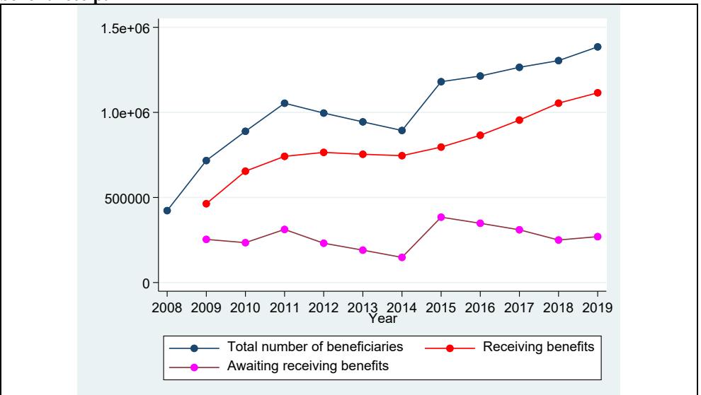
Source: own work using data from Imserso. Instituto de Mayores y Servicios Sociales :: Estadística mensual
Figure A3. Evolution of the number of beneficiaries of the SAAD by dependency degree Note: This figure illustrates the evolution of the number of SAAD beneficiaries, both in total and by degree of dependency. The count of individuals recognized with a moderate degree of dependency begins in 2011, reflecting the gradual inclusion of the least severe dependency category into the SAAD.
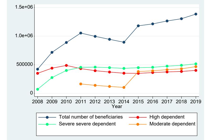
Source: own work using data from Imserso. Instituto de Mayores y Servicios Sociales :: Estadística mensual Figure A4. Evolution of long-term care expenditure with respect to GDP and percentage of SAAD beneficiaries with respect to total population Note: This figure illustrates the evolution of SAAD coverage, showing the percentage of beneficiaries relative to the total Spanish population alongside the percentage of LTC expenditure relative to GDP.
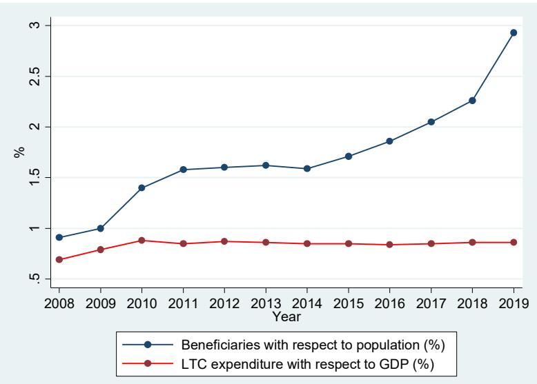
Figure A5. Event-study of the effect of access to long term care services and supports on health and wellbeing with semester calendar data for all years
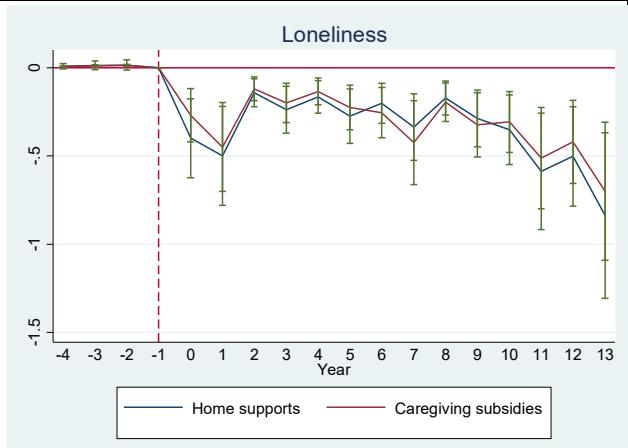
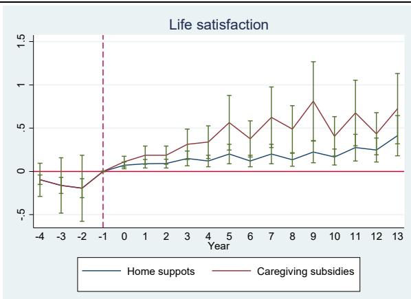
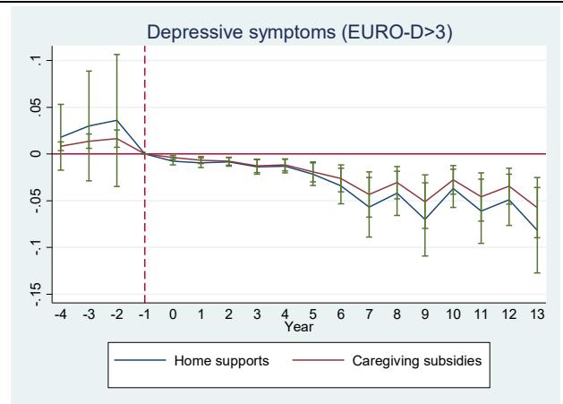
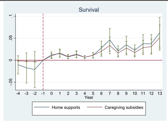
Note: This table displays the event study coefficients of the four outcomes of interest for individuals receiving care subsidies and home care supports. Period 0: implementation of SAAD. Period -4 corresponds to semester to semester to semester semester 2006; 0 to semester 2007. Periods 1 to 13 corresponds to the situation after SAAD by semesters. Source: Own work using SHARE.
Figure A6. Sensitivity test for the parallel trend assumption
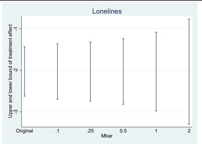
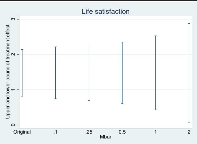
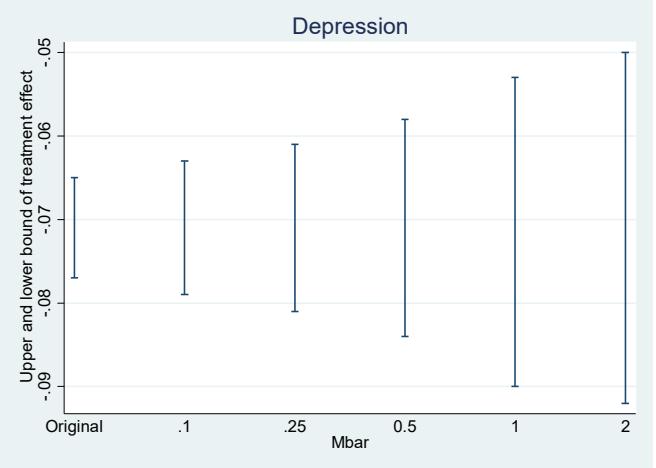
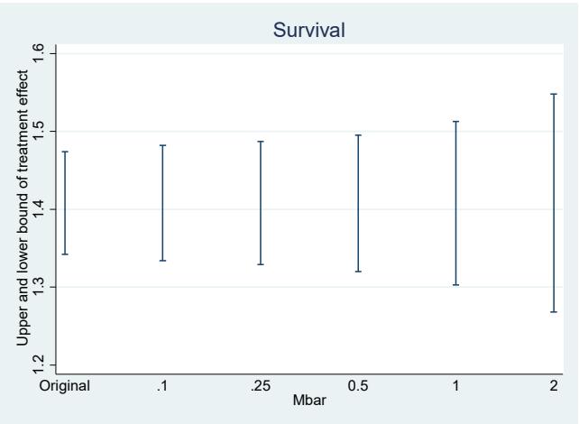
Note: Sensitivity analysis of the parallel trend assumption based on Rambachan and Roth (2023). The figure shows the original estimate and estimates sensitive to violations of the common post-SAAD trend equal to 01. 0.25, 0.5, 1, 1.5 and 2 times the maximum deviation observed in the pre-SAAD period.
Figure A7. Comparison of estimated coefficients for “caregiving subsidies SAAD” and “home supports SAAD” estimating Eq.2 with yearly time dummies or semester time dummie
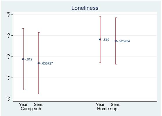
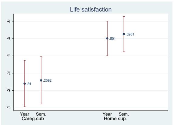
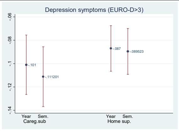
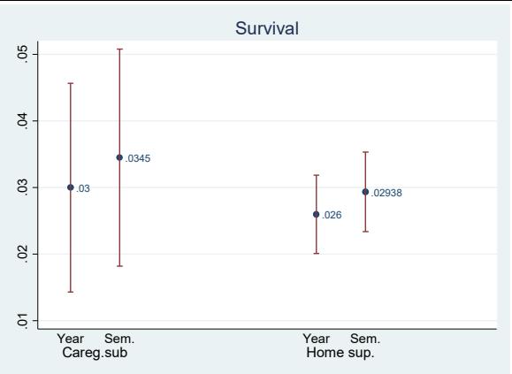
Each dot represents the estimated effect for the corresponding outcome according to equation 3 (proposed model) with year fixed effects (original model) or with semester time dummies.
Table A1. Heterogeneity. Gender and age. OLS-DiD. CEM corrected sample
| Loneliness | Life satisfaction | Depression (Euro-D>3) | Survival | |
| Men | ||||
| Disability allowance | -1.082*(0.590) | 0.025(0.084) | -0.002(0.006) | 0.002(0.014) |
| Caregiving subsidy (SAAD) | -0.601***(0.072) | 0.152**(0.061) | -0.105***(0.011) | 0.008**(0.003) |
| Home care supports (before SAAD) | 1.212(0.882) | 0.034(0.070) | 0.042(0.035) | -0.002(0.011) |
| Home care supports (SAAD) | -0.435***(0.066) | 0.408***(0.056) | -0.073***(0.010) | 0.013***(0.003) |
| F | 21.990 | 36.643 | 13.448 | 39.342 |
| p | 0.000 | 0.000 | 0.000 | 0.000 |
| R2 | 0.335 | 0.350 | 0.326 | 0.389 |
| Women | ||||
| Disability allowance | -0.094***(0.031) | 0.034(0.080) | -0.045***(0.040) | -0.023(0.016) |
| Caregiving subsidy (SAAD) | -0.621***(0.075) | 0.306***(0.073) | -0.098***(0.014) | 0.046***(0.011) |
| Home care supports (before SAAD) | -0.529(0.501) | 0.074(0.209) | 0.019(0.110) | -0.002(0.005) |
| Home care supports (SAAD) | -0.582***(0.049) | 0.571***(0.047) | -0.097***(0.010) | 0.036***(0.003) |
| F | 43.792 | 75.647 | 22.227 | 28.785 |
| p | 0.000 | 0.000 | 0.000 | 0.000 |
| R2 | 0.352 | 0.310 | 0.331 | 0.383 |
| Age 50-64 | ||||
| Disability allowance | -0.526(0.541) | 0.054(0.077) | 0.029(0.018) | 0.049(0.058) |
| Caregiving subsidy (SAAD) | -0.719***(0.068) | 0.357***(0.061) | -0.121***(0.011) | 0.027***(0.004) |
| Home care supports (before SAAD) | -0.491 | 0.506(0.441) | 0.050(0.047) | -0.022(0.017) |
| Home care supports (SAAD) | -1.616 | 0.165***(0.045) | -0.034***(0.013) | 0.027***(0.003) |
| F | 18.898 | 28.325 | 13.004 | 18.477 |
| p | 0.000 | 0.000 | 0.000 | 0.000 |
| R2 | 0.239 | 0.278 | 0.229 | 0.268 |
| Age 65-79 | ||||
| Disability allowance | -0.102***(0.046) | 0.074(0.057) | 0.178***(0.043) | 0.005(0.017) |
| Caregiving subsidy (SAAD) | -0.705***(0.068) | 0.183**(0.078) | -0.087***(0.016) | 0.012**(0.005) |
| Home care supports (before SAAD) | 0.678(0.671) | 0.054(0.047) | -0.004(0.002) | -0.019(0.014) |
| Home care supports (SAAD) | -0.398***(0.062) | 0.616***(0.061) | -0.119***(0.012) | 0.013***(0.004) |
| F | 29.472 | 54.372 | 20.847 | 15.375 |
| p | 0.000 | 0.000 | 0.000 | 0.000 |
| R2 | 0.250 | 0.213 | 0.241 | 0.256 |
| Age 80 and older | ||||
| Disability allowance | 0.007(0.017) | 0.025(0.037) | 0.049(0.129) | -0.015(0.026) |
| Caregiving subsidy (SAAD) | -0.793***(0.171) | 0.410**(0.183) | -0.109***(0.036) | 0.056***(0.022) |
| Home care supports (before SAAD) | -0.294(0.665) | -0.001(0.006) | 0.055(0.067) | -0.007(0.009) |
| Home care supports (SAAD) | -0.473***(0.087) | 0.395***(0.064) | -0.062***(0.013) | 0.028***(0.006) |
| F | 16.619 | 35.359 | 27.065 | 37.285 |
| p | 0.000 | 0.000 | 0.000 | 0.000 |
| R2 | 0.252 | 0.252 | 0.233 | 0.356 |
Note: This table presents the estimated coefficients for the four outcomes analyzed using a difference-in-differences model with OLS on the sample obtained after applying coarsened exact matching (CEM), differentiated by sex and age cohort. Covariates correspond to those in M4 of Table 2, excluding variables related to the heterogeneity dimension under study. Standard errors, shown in parentheses, are clustered at the regional level and obtained using a block bootstrap with 1,000 replications. Statistical significance is indicated as , and
Table A2. Heterogeneity. Residence. OLS-DiD estimates. CEM corrected sample
| Loneliness | Life satisfaction | Depression (Euro-D>3) | Survival | |
| Lives in rural area | ||||
| Disability allowance | 0.077(0.138) | 0.053(0.201) | -0.134***(0.028) | 0.062(0.076) |
| Caregiving subsidy (SAAD) | -1.677***(0.159) | 0.946***(0.249) | -0.350***(0.075) | 0.083***(0.027) |
| Home care supports (before SAAD) | 0.496(0.984) | 0.123(0.211) | -0.024(0.094) | 0.004(0.093) |
| Home care supports (SAAD) | -0.553***(0.041) | 0.541***(0.039) | -0.096***(0.022) | 0.133***(0.020) |
| F | 13.902 | 27.949 | 17.625 | 26.022 |
| p | 0.000 | 0.000 | 0.000 | 0.000 |
| R2 | 0.364 | 0.139 | 0.348 | 0.415 |
| Does not live in rural area | ||||
| Disability allowance | -0.237(0.535) | 0.151(0.221) | -0.132***(0.032) | 0.009(0.014) |
| Caregiving subsidy (SAAD) | -0.607***(0.055) | 0.268***(0.052) | -0.099***(0.010) | 0.040***(0.010) |
| Home care supports (before SAAD) | -0.330(0.474) | 0.153(0.281) | -0.151***(0.023) | 0.027(0.024) |
| Home care supports (SAAD) | -0.373***(0.116) | 0.404***(0.102) | -0.088***(0.008) | 0.040***(0.003) |
| F | 58.503 | 139.803 | 41.185 | 84.780 |
| p | 0.000 | 0.000 | 0.000 | 0.000 |
| R2 | 0.345 | 0.132 | 0.337 | 0.310 |
| Lives alone | ||||
| Disability allowance | -0.255***(0.421) | -0.001(0.004) | 0.170***(0.030) | 0.005(0.013) |
| Caregiving subsidy (SAAD) | -0.761***(0.174) | 1.155**(1.951) | -0.266***(0.057) | 0.040***(0.012) |
| Home care supports (before SAAD) | 0.328(0.501) | 0.255(0.178) | 0.100***(0.025) | 0.034***(0.010) |
| Home care supports (SAAD) | -0.584***(0.043) | 0.514***(0.038) | 0.085***(0.008) | 0.032***(0.003) |
| F | 56.602 | 81.890 | 34.805 | 33.497 |
| p | 0.000 | 0.000 | 0.000 | 0.000 |
| R2 | 0.243 | 0.282 | 0.232 | 0.340 |
| Does not live alone | ||||
| Disability allowance | 0.205(0.187) | 0.050(0.087) | 0.114(0.111) | 0.018(0.043) |
| Caregiving subsidy (SAAD) | -0.590***(0.055) | 0.250***(0.049) | -0.099***(0.009) | 0.021**(0.009) |
| Home care supports (before SAAD) | -1.059(0.881) | 0.042(0.080) | 0.007(0.006) | 0.024(0.022) |
| Home care supports (SAAD) | -0.301***(0.097) | 0.520***(0.107) | -0.098***(0.018) | 0.022***(0.004) |
| F | 4.813 | 4.601 | 6.823 | 225.391 |
| p | 0.000 | 0.000 | 0.000 | 0.000 |
| R2 | 0.030 | 0.033 | 0.044 | 0.573 |
Note: his table presents the estimated coefficients for the four outcomes analyzed using a difference-in-differences model with OLS on the sample obtained after applying coarsened exact matching (CEM), differentiated by place of residence and household size. Covariates correspond to those in M4 of Table 2, excluding variables related to the heterogeneity dimension under study. Standard errors, shown in parentheses, are clustered at the regional level and obtained using a block bootstrap with 1,000 replications. Statistical significance is indicated as *p < 0.10, **p < 0.05, and ***p < 0.01.
Table A3. Heterogeneity. Dependency. OLS estimates. CEM corrected sample
| Loneliness | Life satisfaction | Depression (Euro-D>3) | Survival | |
| Moderate dependent | ||||
| Disability allowance | 0.083(0.307) | 0.117(0.080) | 0.021(0.046) | 0.023(0.101) |
| Caregiving subsidy (SAAD) | -0.024(0.034) | 0.299(0.229) | 0.020(0.161) | 0.237(0.262) |
| Home care supports (before SAAD) | -0.991(1.236) | 0.167(0.120) | 0.035(0.074) | -0.021(0.073) |
| Home care supports (SAAD) | -0.190(0.117) | -0.113(0.334) | -0.007(0.026) | 0.039(0.044) |
| F | 3.694 | 10.395 | 13.392 | 16.431 |
| p | 0.000 | 0.000 | 0.000 | 0.000 |
| R2 | 0.238 | 0.240 | 0.241 | 0.242 |
| Severe dependent | ||||
| Disability allowance | -0.154(1.635) | 0.180(0.107) | -0.017(0.216) | 0.393*(0.180) |
| Caregiving subsidy (SAAD) | -0.557**(0.263) | 1.055****(0.229) | -0.095****(0.023) | 0.063**(0.034) |
| Home care supports (before SAAD) | 1.847(1.627) | 0.033(0.067) | 0.087(0.124) | -0.097(0.109) |
| Home care supports (SAAD) | -0.294*(0.179) | 0.377**(0.154) | -0.071**(0.027) | 0.052***(0.012) |
| F | 35.293 | 53.063 | 15.781 | 12.990 |
| p | 0.000 | 0.000 | 0.000 | 0.000 |
| R2 | 0.381 | 0.324 | 0.363 | 0.353 |
| High dependent | ||||
| Disability allowance | -0.805(1.977) | 0.120(0.091) | -0.089(0.218) | -0.062(0.175) |
| Caregiving subsidy (SAAD) | -0.597***(0.176) | 0.248***(0.078) | -0.122*(0.067) | 0.027***(0.008) |
| Home care supports (before SAAD) | 2.380(1.975) | 0.027(0.068) | -0.034(0.154) | 0.159(0.123) |
| Home care supports (SAAD) | -0.270***(0.102) | 0.217***(0.050) | -0.111***(0.050) | 0.027***(0.009) |
| F | 22.408 | 21.205 | 20.654 | 16.749 |
| p | 0.000 | 0.000 | 0.000 | 0.000 |
| R2 | 0.248 | 0.265 | 0.228 | 0.259 |
Note: This table presents the estimated coefficients for the four outcomes analyzed using a difference-in-differences model with OLS on the sample obtained after applying coarsened exact matching (CEM), differentiated by dependency degree (approximated using Katz’s Index). Covariates correspond to those in M4 of Table 2, excluding variables related to the heterogeneity dimension under study. Standard errors, shown in parentheses, are clustered at the regional level and obtained using a block bootstrap with 1,000 replications. Statistical significance is indicated as *p < 0.10, **p < 0.05, and
Table A4. Heterogeneity. Income and Wealth. OLS-DiD estimates. CEM corrected sample
| Loneliness | Life satisfaction | Depression (Euro-D>3) | Survival | |
| Lowest income quintile | ||||
| Disability allowance | -0.003(0.010) | 0.022(0.020) | -0.159**(0.064) | -0.012(0.028) |
| Caregiving subsidy (SAAD) | -1.040***(0.159) | 0.588***(0.157) | -0.163***(0.026) | 0.056***(0.015) |
| Home care supports (before SAAD) | 0.888(0.925) | 0.055***(0.019) | -0.093**(0.047) | 0.017(0.021) |
| Home care supports (SAAD) | -1.981**(0.926) | 0.592***(0.123) | -0.166***(0.056) | 0.043***(0.007) |
| F | 29.334 | 15.326 | 29.713 | 56.928 |
| p | 0.000 | 0.000 | 0.000 | 0.000 |
| R2 | 0.343 | 0.388 | 0.344 | 0.339 |
| Highest income quintile | ||||
| Disability allowance | -1.023(0.715) | 0.089(0.051) | -0.014(0.035) | -0.004(0.026) |
| Caregiving subsidy (SAAD) | -0.503***(0.113) | 0.412***(0.091) | -0.101***(0.019) | 0.005(0.008) |
| Home care supports (before SAAD) | 1.082(1.011) | 0.079(0.067) | 0.069(0.048) | 0.032(0.020) |
| Home care supports (SAAD) | -0.368***(0.090) | 0.314***(0.068) | -0.099***(0.020) | 0.030***(0.006) |
| F | 22.393 | 25.286 | 29.006 | 53.775 |
| p | 0.000 | 0.000 | 0.000 | 0.000 |
| R2 | 0.255 | 0.221 | 0.238 | 0.396 |
| Lowest wealth quintile | ||||
| Disability allowance | -1.256(1.939) | -0.124(0.223) | 0.094(0.066) | 0.014(0.027) |
| Caregiving subsidy (SAAD) | -1.605***(0.121) | 0.598***(0.107) | -0.196***(0.021) | 0.041***(0.015) |
| Home care supports (before SAAD) | -0.384(1.123) | 0.184(0.093) | -0.004(0.008) | 0.022(0.022) |
| Home care supports (SAAD) | -1.497***(0.109) | 0.630***(0.101) | -0.118***(0.020) | 0.033***(0.007) |
| F | 38.896 | 18.103 | 38.961 | 71.727 |
| p | 0.000 | 0.000 | 0.000 | 0.000 |
| R2 | 0.341 | 0.394 | 0.342 | 0.356 |
| Highest wealth quintile | ||||
| Disability allowance | -0.776(0.591) | 0.017(0.030) | -0.256***(0.060) | 0.132(0.155) |
| Caregiving subsidy (SAAD) | -0.751***(0.137) | 0.302***(0.129) | -0.070***(0.024) | 0.026***(0.006) |
| Home care supports (before SAAD) | -1.635(1.901) | 0.041(0.055) | -0.154***(0.046) | 0.010(0.010) |
| Home care supports (SAAD) | -0.541***(0.087) | 0.228***(0.079) | -0.055***(0.015) | 0.036***(0.006) |
| F | 17.961 | 33.274 | 29.191 | 65.985 |
| p | 0.000 | 0.000 | 0.000 | 0.000 |
| R2 | 0.275 | 0.267 | 0.240 | 0.327 |
Note: This table presents the estimated coefficients for the four outcomes analyzed using a difference-in-differences model with OLS on the sample obtained after applying coarsened exact matching (CEM), differentiated by household income and wealth. Covariates correspond to those in M4 of Table 2, excluding variables related to the heterogeneity dimension under study. Standard errors, shown in parentheses, are clustered at the regional level and obtained using a block bootstrap with 1,000 replications. Statistical significance is indicated as and
Appendix B
Table B1. Explanatory variables
| Categories | Definition |
| Socio-demographic variables | ○ Age and age squared.○ Gender○ Level of education. Education is categorized in four levels using the 1997 International Standard Classification of Ed Este texto se ha extraído automáticamente del documento original. Para citarlo o leerlo con su maquetación, descargue el PDF. Descargar en PDF |