A debt brake expenditure rule for the Spanish regions
FERNANDO GONZÁLEZ GONZÁLEZDIEGO MARTÍNEZ LÓPEZ
Fedea Policy Paper 2026/02
Junio de 2026
fedea
Las opiniones recogidas en este documento son las de sus autores y no coinciden necesariamente con las de Fedea.
Fernando González González
Diego Martínez López**
Abstract
This paper proposes a new expenditure rule applicable to Spanish Autonomous Communities (ACs) that aims at achieving a predictable debt reduction path. The paper draws on existing contributions based on the "debt brake" concept, adapting them to the reality of Spanish ACs. Particularly, the proposal consists of an expenditure rule benchmarked against a projection of smoothed past AC revenues, adjusted by a debt-reduction parameter. The proposed rule presents feature that the literature of fiscal rule considers desirable, and addresses problems related to the application of the Spanish expenditure rule. Simulations show how this rule would limit expenditure growth and reduce Autonomous Communities’ debt against official rules, when applied over different time periods and considering a constellation of parameters relative to the debt adjustment and revenue-raising incentives.
Keywords: public deficit, public debt, fiscal rules, expenditure rule, Autonomous Communities. JEL Classification: H70, H74.
WP version. We thank the research assistance provided by Pablo Porrero Ramírez. We acknowledge the financial support by the Instituto de Estudios sobre la Hacienda Pública Andaluza under its VI Research Program. Both the text and any remaining errors are the sole responsibility of the authors and do not reflect the views of any of the funders or institutions they belong to.
* Complutense University of Madrid.
** Pablo Olavide University at Seville and FEDEA.
1. Introduction
The surge in what is known as “second-generation fiscal rules”, i.e. those fiscal rules that aimed at strengthening enforceability while ensuring flexibility (Eyraud et al, 2018), was a global trend, especially at the EU level and also in Spain, after the financial crises. These second-generation fiscal rules have led to fiscal consolidation, significantly reducing deficits after the financial crisis, but at the cost of increasing indebtedness, reducing public investment (Delgado-Tellez et al, 2020) and increasing complexity of the fiscal responsibility frameworks. In this context, the global rise in public debt levels may be due to poor compliance with fiscal rules but also to ill-designs and institutional frameworks related to these fiscal rules, which have led to pro-cyclical fiscal policies.
After the pandemic and the worldwide phasing-out of escape clauses, fiscal rules are being reinstated. The European Union launched a new legislative package that aimed at introducing enhanced flexibility on the application of fiscal rules1. Countries with high levels of debt will have individual fiscal adjustment paces to be framed in multiannual fiscal plans of 4 to 7 years, depending on the structural reforms agreed and investments in priority areas, such as green transition and digitalization. Additionally, countries with a debt level above certain levels will have to face a minimum structural adjustment, in order to reach the targets.
There is consensus that new fiscal rule frameworks must address a completely different context than the so-called second-generation rules’ frameworks, targeting more closely the debt reduction objective (AIReF, 2025). Additionally, the design of fiscal rules in subnational governments require specific considerations and literature does not offer clear guidance on the best conceptual framework for subnational institutional arrangements, including fiscal rules, often paying little attention to the specific challenges posed by decentralized contexts (Eyraud et al, 2020).
In this respect, this paper offers a conceptual framework for establishing a new expenditure rule for the Autonomous Communities (ACs) in Spain that addresses their current challenges. ACs rank among the most indebted subnational governments in the EU and in the world. The regional fiscal governance framed in the LOEPSF has not been very effective in terms of debt sustainability (Martínez-López, 2020). After more than 4 years without fiscal rules or fiscal objectives, fiscal rules have been reactivated in Spain, but the time is ripe for a new fiscal rules framework that responds to the new reality of high debt. Our proposal takes into account the problem of public debt sustainability in a context where interest rates are still high, and post-pandemic debt levels are unprecedented.
The approach essentially presents a fiscal rule consistent with a normative reduction of the stock of public debt as percentage of GDP to a pre-set level and at a certain convergence speed. In a sense, it can be seen as a debt brake. This work expands on previous proposals, particularly that of González and Martínez-López (2021), exploring a specific type of fiscal rule, the expenditure rule, which, according to the literature on the subject of fiscal rules, has certain advantages over other types of fiscal rules (Brändle and Elsener, 2024). Furthermore, it seeks to address certain problems related to the dynamics of the expenditure rule in Spain, such as that of expenditure consolidations, as well as the slackness in the enforcement system at non-compliance, laying out both a mid-term fiscal balance and a credible and predictable debt reduction path.
1 See the legal texts published in the Official Journal of the European Union on EUR-Lex:
https://eur-lex.europa.eu/eli/reg/2024/1263/oj
https://eur-lex.europa.eu/eli/dir/2024/1265/oj
https://eur-lex.europa.eu/eli/reg/2024/1264/oj
The paper also contributes to the current literature on fiscal rules of subnational governments by proposing an expenditure rule linked to a variable that lies more under the control of regional governments, their own revenues (“non-financial resources”). This way, it moves away from the usual reference applied in national expenditure rules, namely the GDP.
The next section provides a brief overview of the main problems identified within the design of the expenditure rule in Spain for Autonomous Communities as established in the Organic Law on Budgetary Stability and Financial Sustainability (LOEPSF in its Spanish acronym). In section 3, we review the literature related to expenditure rules and previous proposals based on a debt brake. We then present in section 4 the general framework of the new rule. Section 5 provides details of the specific methodology and data used for Spanish ACs. In section 6, results are shown, with different simulation exercises to assess the performance of this rule at the period immediately before the pandemic, at a more recent period when ACs are closer to fiscal balance, and with different specifications of the rule and forecasting parameters; here, our findings have been also compared with fiscal outcomes that resulted from applying the official rules. Section 7 provides some extensions regarding some ways to manage the stringency of the rule. A final section summarizes the main conclusions.
2. The expenditure rule in Spain. The Case of the Autonomous Communities
According to the expenditure rule in Article 12 of the LOEPSF, the growth of computable spending by the Spanish Public Administrations is limited to the medium-term growth of GDP. Computable spending is defined as non-financial outlays, excluding debt interest and other nondiscretionary expenses or those financed by transfers from other administrations. Computable spending may be adjusted upwards or downwards to reflect regulatory changes that result in permanent revenue increases or decreases, respectively.
As noted by Spanish Independent Fiscal Institution (2016, 2024, 2025), called AIReF using its Spanish acronym, and similarly to other European fiscal rules (European Fiscal Board, 2019), the current formulation of the expenditure rule does not allow for an adequate approach toward the medium-term objective (in terms of public debt). At best, compliance with the current expenditure rule leads to a neutral fiscal policy stance, which is insufficient to reduce substantially public debt, particularly given the high structural deficits experienced in recent years.
Furthermore, the current configuration of the rule, especially in terms of its application, has led to compliance issues. Specifically, measuring compliance based on settled budgets, without any form of adjustment in subsequent fiscal years to ensure the return to the long-term benchmark, generates considerable problems. In other words, a significant initial non-compliance allows administrations to "live off the non-compliance" as there is no correction of the maximum growth rate for the years to come (Fernández-Huertas et al, 2026). Similarly, if the rule is met and spending remains below the maximum set by the rule, the capacity for spending in subsequent years is restricted, creating incentives to either breach the rule or remain as close to the limit as possible. AIReF has repeatedly expressed concern with this method of measuring compliance with the expenditure rule (AIReF, 2016).
Moreover, breaching the expenditure rule only entails drafting a not very strict financial-economic plan (PEF in its Spanish acronym) to be met over a period shorter than two years. This plan assesses compliance taking as reference the expenditure in the settled budget, ignoring specific measures to ensure return to the compliance trend in the following year. This makes noncompliance relatively easy to assume in practice.
On top of these problems, we also note issues related to the other fiscal rules applicable to ACs in Spain, most notably, the absence of explicit methodology to set fiscal targets in terms of public balance and to estimate debt reduction targets for ACs. The lack of an effective coordination among the functioning of different rules (González and Martínez-López, 2021) or coherence with the equivalent EU level rules (see AIReF, 2025, for a discussion on the lack of coherence between the Spanish expenditure rule and EU fiscal rules) are additional caveats of the current economic governance framework in Spain.
3. Literature with discussion
Fiscal rules have been increasingly adopted over the last 20 years. As increased fiscal pressure and risks urge countries to address the public debt legacy left by recent economic crises, fiscal rules come under greater scrutiny. Depending on the type of fiscal variables on which they focus (Eyraud et al, 2020), the most common rules include debt rules (ceilings on the debt-to GDP-ratio), deficit or nominal balance rules (constraint on the size of the deficit or requesting nominal balance), revenue rules (ceiling or floor on revenues) and expenditure rules (ceiling on levels/growth of spending). In addition, structural balance rules are sometimes defined as a way to consider the business cycle. Fiscal rules can be also supplemented with a debt correction mechanism (“debt brake”) to correct for past deviations from the target.
Brändle and Elsener (2024) carried out a survey on evidence related to the functioning of fiscal rules and their importance for sound and sustainable fiscal policies. They find that fiscal rules are positively related to improvements in fiscal performance and reductions in public debt public spending volatility. Furthermore, the fiscal rules lead to more accurate budget forecasts and better sovereign bond ratings. The available evidence also suggests that a country's ability to respond to adverse shocks depends primarily on whether it has sufficient fiscal space, in which the design of the rules can also play a supportive role (Medas and González, 2023).
Three properties are normally expected from fiscal rules: simplicity, enforceability and flexibility (Eyraud et al, 2018). The first one, simplicity, means that the rule should be based on observable variables, without resorting to estimations. The second property, enforceability, implies that there should be enforcement mechanisms, such as corrective measures, and these should be designed in a way to ensure that compliance with the rule is feasible. Finally, flexibility means that the rule must be able to cope with different fiscal situations, both in terms of the economic cycle and in terms of exceptional circumstances, such as, for example, a pandemic.
Complex rules, such as structural balance rules, that aim at introducing countercyclical properties to the rule, are good at responding to the economic cycle. However, the property of simplicity is sacrificed as typically also requires estimating an output gap, which makes it difficult to operate, communicate, and monitor the system (Andrle et al, 2015).
Simplicity can be undermined also by a framework with multiple rules. Using a sample composed of 27 EU Member States for a period spanning 2000 to 2021, Cǎpraru and Sprincean (2025) find that countries’ compliance with fiscal rules is positively associated with the number of numerical fiscal targets. However, this association only holds up to a specific threshold. Once this threshold is achieved, the relationship becomes negative, implying that the multiplication of numerical fiscal rules may undermine compliance, thereby reducing their effectiveness.
In the context of flexibility, the available evidence suggests that a country's ability to respond to adverse shocks depends primarily on whether it has sufficient fiscal space, although the design of the rules can also play a supportive role (Medas and González, 2023). In a different context, flexibility mechanisms such as well-defined escape clauses or means to adapt to economic downturns are particularly relevant. In recent years, many countries have enhanced their fiscal rules by adding escape clauses to allow for greater flexibility (Eyraud et al, 2018). Prior to the COVID-19 pandemic, two-thirds of countries with fiscal rules had included escape clauses; in fact, their number doubled in the early 2000s.
Finally, the discussion on the fiscal rules may present critical issues at the phase of enforceability, such as those signaled above in the case of the Spanish expenditure rule, which are more related to the design of corrective measures and the play of incentives for compliance. Based on data from 74 countries from the years between 1985 and 2012, Badinger and Reuter (2017) found that countries with more rigorous fiscal rules show a better budgetary balance, lower interest rate spread for bonds and lower GDP volatility. Drawing on the latest updates to the IMF’s Fiscal Rules and Fiscal Councils databases, which cover more than 120 economies, Alonso et al (2025) propose new indices to quantify the overall strength of fiscal rules and the institutional quality of fiscal councils. They find significant cross-country variation and a positive correlation between the strength of rules and fiscal discipline.
In general, there is a consensus in the literature on the fact that there are trade-offs in achieving simultaneously the three properties, when we look at the current sets of fiscal rules. Complex rules that can be applied to multiple contexts tend to lack transparency. Simple transparent rules tend not to fit all economic situations or exhibit problems at the enforcement phase.
When designing fiscal rules at the subnational level, certain particularities need to be considered as well. Eyraud et al (2020) discussed types of rules and design aspects to bear in mind in subnational level contexts. The literature has traditionally identified questions such as informationrelated problems and the consequent agency theory-related issues in the relationship with the central government, or budget rigidities in their expenditure preventing them from using discretionary fiscal policy in the same way as the central government.
One of the primary hurdles at the subnational level is the lack of timely and reliable data. This shortage of robust information systems may make countries prefer certain fiscal rules (for example, debt rules) over other types because debt data may be available more frequently and promptly than complex deficit or expenditure metrics. Similarly, the difficulty of measuring the output gap at subnational level may also have an impact on the rules applicable to SNGs, avoiding cyclically adjusted balance rules. In some cases, subnational governments use simpler, less precise tools like expenditure growth limits or "Rainy Day Funds" to handle economic swings (Tax Policy Center, 2024).
There is also a clear "principal-agent" problem between the central government and subnational entities. When large tax and expenditure responsibilities are decentralized, the central government (the principal) may find it impossible to monitor how efficiently local governments (the agents) utilize those taxes, resulting in moral hazard. Furthermore, subnational governments often face "vertical externalities," where their local fiscal problems are transmitted upward to the national level through higher risk premiums on sovereign debt or the direct cost of bailout payments (Martínez-López, 2022).
The literature also refers to the common pool problem of subnational governments as they may be more prone to deficit bias because they often operate under a "soft budget constraint" (Baskaran, 2012). This happens when local authorities expect to receive gap-filling transfers from the national government if they run into trouble (Goodspeed, 2017). Additionally, because they often finance local spending with transfers funded by taxpayers from other jurisdictions, they fail to internalize the full cost of their expenditures—a classic "common pool" problem. This creates, under certain circumstances, a much higher incentive to overspend and borrow excessively compared to the national level.
Finally, subnational governments may face more budget rigidity and structural pressures than a national government, which has more room to reallocate resources. Subnational budgets are notoriously rigid since they are typically responsible for essential, politically sensitive services like education, health, and social protection. When a shock occurs, they cannot easily cut these programs, making it much harder for them to comply with strict fiscal limits without external help or flexible "escape clauses". A clear example of this occurred during the COVID-19 pandemic. The crisis generated a 'scissors effect' on subnational finances, forcing central governments worldwide to implement exceptional financial support measures, massive grants, and the temporary relaxation of fiscal rules to prevent local governments from collapsing under the weight of their essential responsibilities (OECD, 2020).
In this paper, we focus on a specific type of fiscal rule, expenditure rules, that is growing in popularity and seems to be associated with good fiscal performance (see Brändle and Elsener, 2024). We can define expenditure rules, following Andrle et al. (2015), as permanent limits on total primary or current spending in absolute terms, real growth rates (or real potential growth), or as a percentage of GDP. These rules are generally transparent (directly constraining the budget).
They inherit many of the macroeconomic stabilization properties of a structural balance rule by allowing automatic stabilizers on the revenue side to fully operate.
Moreover, adequate specification of these rules (for instance, in terms of real growth rather than as a percentage of GDP) tends to further support macroeconomic stabilization. While they are not directly linked to the debt sustainability objective (since they do not constrain the revenue side), they can trigger necessary fiscal consolidation consistent with fiscal sustainability when accompanied by a debt brake. Focusing on expenditure rules, Cordes et al (2015) presented an analysis for 29 advanced and developing countries for the period 1985–2013. Using a dynamic panel estimation approach, the analysis showed that these rules were associated with better spending control, countercyclical fiscal policy and improved fiscal discipline. The authors also suggested that expenditure rules were associated with lower public expenditure volatility and higher public investment efficiency.
Comparative evidence shows a clear upward trend in the adoption of these rules: since the late 1980s, the number of countries using expenditure rules has grown from fewer than 10 to approximately 55 countries by 2021 (Davoodi et al, 2022). This growth is driven largely by advanced economies, although many emerging and developing nations have also adopted them. Thus, expenditure rules are being increasingly used as "operational rules" to support long-term debt rules, providing a more practical guide for annual budgeting. Despite their benefits, the existing evidence also highlights specific challenges. The most important one is the fact that, as signaled above, expenditure rules are not directly linked to debt sustainability because they do not consider the revenue side of the budget. That is why the literature on fiscal rules has explored the inclusion of debt brakes in fiscal rules, in order to target explicitly the debt reduction long-term goal.
Regarding debt brakes, Andrle et al (2015) presented different specifications of a debt brake inserted in different rules for a proposal at the EU level. Their paper argued for moving from the Six Pack and Two Pack governance architecture of fiscal rules to a two-pillar approach with a single fiscal anchor (the public debt-to-GDP ratio) and a single operational target (an expenditure growth rule, possibly with an explicit debt brake, that is, a formal and deterministic debt-correction mechanism) linked to the anchor. They assessed the ability of three operational rules—the overall (nominal) balance, the structural balance, and real expenditure growth—to deliver macroeconomic stabilization in the form of debt sustainability. It was done based on stochastic simulations that were applied to a stylized model of a euro area economy and evaluating how different operational rules performed over the course of the business cycle.
The specific form for the balance fiscal rule considering the effects of the business cycle can be derived from this general expression:
\[D e f _ {t} = D e f ^ {*} - \alpha (O u t p u t G a p _ {t}) - \beta (D e b t _ {t - 1} - D e b t ^ {*})),\tag{1}\]
where the deficits and debt are relative to GDP, in percentage, and the output gap is relative to the level of potential output, in percentage as well. represents the fiscal deficit in the current period and the benchmark value of the deficit, i. e., the long-term deficit target.
The coefficient α determines the sensitivity of the deficit to the output gap. In a nominal balance rule, α is set to meaning the deficit target does not change regardless of whether the economy is in a boom or a recession. Under a structural balance rule, α is positive (calibrated later at 0.45 in this paper), allowing the deficit to expand or contract to act as an economic stabilizer. The debt correction mechanism acts through This term acts as a "debt brake". It adjusts the current deficit based on how far the previous year's debt deviated from the long-term debt anchor
With respect to the expenditure growth rule, Andrle et al (2015) follow the next expression:
\[1 0 0 \times l o g (E x p _ {\mathrm{t}}) = 1 0 0 \times l o g \big (\alpha Y _ {\mathrm{t}} ^ {*} \big) - \beta (d e b t _ {t - 1} - D e b t ^ {*}),\tag{2}\]
where is the level of public expenditure consistent with the difference between the potential output and distance of public debt to its value of long-term anchor. By linking the log of expenditures to the log of potential output , the rule mandates that expenditure growth partially follows potential output growth. The factor of 100 is used to convert these logarithmic differences into standard percentage points. While the first part of the formula aligns spending with the economy's trend growth, the second part, , acts as the "debt brake". It forces the expenditure growth rate to slow down if the debt from the previous period is higher than the long-term anchor , ensuring the sustainability of public finances.
González and Martínez-López (2021) proposed a similar setting with an anchor variable (or final objective) in terms of public debt and an instrumental variable such as the expenditure rule. It aims at approximating the debt to a normative reference value. In general, an expenditure rule as a growth rate of public spending designed to address this dual perspective would be defined as follows:
\[E R _ {t} = F [ \mu Y _ {t} ^ {*}, \delta (D e b t _ {t - 1} - D e b t _ {t} ^ {*}) ],\tag{3}\]
where is the potential output and its weight in the expenditure rule. is the gap between the existing debt stock and the normative reference debt stock denoted by an asterisk, with being the weight given to this debt gap when calculating the expenditure rule. The partial derivative of with respect to the first argument is positive, and negative with respect to the second argument. Thus, the first argument of reflects the focus on ensuring counter-cyclical properties, while the second one addresses potential sustainability issues arising from excess debt, both weighted accordingly.
In such a design, real public spending follows potential output while maintaining a focus on the required fiscal consolidation to reduce the debt stock. Referring public spending growth to potential output provides the rule with stabilization properties. In expansion periods with positive output gaps, the difference between revenues and real public spending will tend to stabilize the economy while at times with negative output gaps real expenditure will grow higher than revenue and will therefore provide a counter-cyclical stimulus.
Martínez-López and González (2021) also proposed a methodology for determining deficit targets with an explicit debt-reduction component for ACs. Based on the former European fiscal governance, they defined the fiscal adjustment required for each AC to bring its given initial public debt stock to a normative reference value according to a specific speed of adjustment.
To derive the proposed fiscal rule, the authors started with the fundamental law of motion for the debt-to-GDP ratio and solved for the required primary balance. The evolution of the debt-to-GDP ratio depends on the interest rate (?), the real growth rate of the economy (?), and the primary balance . The standard equation is then:
\[D e b t _ {t} - D e b t _ {t - 1} = (r - g) D e b t _ {t - 1} - S _ {t}\tag{4}\]
A debt-reduction rule mandates that the change in debt must be equal to a fraction α of the distance between the current debt and the long-term target (????∗):
\[D e b t _ {t} - D e b t _ {t - 1} = - \alpha (D e b t _ {t - 1} - D e b t ^ {*})\tag{5}\]
The parameter ? is interpreted as the speed of convergence of public debt towards its benchmark value. This ensures that if debt is above the target, the government must take action to reduce it. To find the surplus (?) required to achieve this specific reduction, we set the two expressions for equal to each other:
\[(r - g) D e b t _ {t - 1} - S _ {t} = - \alpha (D e b t _ {t - 1} - D e b t ^ {*})\tag{6}\]
Finally, we rearrange the terms to isolate the surplus on one side:
\[S _ {t} = (r - g) D e b t _ {t} + \alpha (D e b t _ {t - 1} - D e b t ^ {*})\tag{7}\]
Higher values for the first term on the right-hand side (debt service payments compared to GDP growth) would require a larger primary surplus. The second term, which captures both the speed of adjustment and the distance from the target debt stock, increases the need for a larger primary surplus. Based on a simulation that covers years 2013-2018, Martínez-López and González (2022) concluded that this rule is not overly demanding in terms of deficit targets for ACs as a whole or on a cross-sectional basis.
This approach has been further updated in Martinez et al (2026). Their new simulations demonstrate that a convergence speed α of 0.05 allows for a gradual reduction of regional debt — from 20.7% in 2025 to 16.4% in 2041— through feasible deficit targets that fluctuate according to potential GDP growth. This refined framework ensures that sub-national fiscal efforts remain consistent with the broader commitments undertaken by the Kingdom of Spain within the new EU economic governance.
In principle, given the structure of the equation ( 7), we would still face the issue of pro-cyclicality in fiscal rules, similar to the European context when this rule would be in place. Note that when economic growth is robust (i.e., ? is high), the required fiscal surplus is smaller, and vice versa. However, it can be argued that macroeconomic stabilization is a function of fiscal policy that is significantly weakened in sub-central contexts. In this regard, Lago et al (2019) question whether fiscal consolidation strategies at the regional level necessarily lead to significant reductions in GDP. They provide evidence for the Spanish case that fiscal multipliers lose their power in subcentral contexts due to the openness and economic integration of regional economies.
For the case of Spain, AIReF (2022) have also proposed a methodology to set a specific debt anchor that generates a feasible reduction path. When establishing this anchor, they consider the initial debt level (present), the historical evolution of the debt ratio (past), and the projected trends of public revenues and expenditures (future), to take into account the implications of the fiscal policy commitments made. Once the debt anchor is set up, its implications for short- and mediumterm fiscal policy are reflected through a primary spending path in levels, net of new revenue measures. This proposal would imply that each elected government proposes to the European institutions, at the beginning of each term, a debt anchor and a spending path derived from it which, being feasible, contributes to a sufficient reduction of the ratio during the legislature. Once approved, this path would be the binding reference in the following four years.
This proposal shares some features with our contribution (such as the enforcement procedure of the 4 years coinciding with the electoral cycle, the consideration of the initial level of debt and the projected trends of public revenues). However, our proposal will try to bring the tailoring of the rule to the specific economic reality of the ACs a step further, by establishing individual differentiated ceilings.
This is precisely in line with the latest proposal of AIReF (2025). In this case, they shift the focus away from annual nominal deficit targets, which have often proven unrealistic or inconsistent, to a net expenditure rule at the center of fiscal supervision. This national expenditure rule should be harmonized with the European framework, specifically tracking net primary expenditure (net of revenue measures) to ensure that the ACs contribute effectively to the sustainability of public debt.
Furthermore, AIReF argues that these fiscal rules should no longer be applied uniformly to every region regardless of their fiscal position. Instead, they propose differentiated reference rates and targets based on each community's specific starting point and feasibility of compliance. For communities with financial imbalances, the expenditure rate should be designed to achieve budgetary equilibrium by the end of a four-year period, provided it remains realistic. To ensure long-term stability and regional "ownership" of these commitments, AIReF also recommends that each Autonomous Community develop its own Medium-Term Structural Fiscal Plan to align their individual budgetary planning with the national and European strategies.
Finally, we have also found other examples of fiscal rules in the form of expenditure rules, which are benchmarked on a revenue basis. In Brazil, wages in the public sector are limited to 50 percent of total revenue of the Federal Government. In Colombia, subnational governments’ current expenditure must not grow above certain thresholds as percentage of their discretionary revenue.
But the most classic example of a dynamic expenditure rule with a revenue-driver is Switzerland. According to Salvi et al. (2020), the Swiss debt containment rule stands out as a clearly defined fiscal rule with a constitutional basis that constrains deviating from a balanced budget in the longterm. In 2001, a large majority of Swiss voters approved the fiscal rule in a public referendum. The rule consists of a simple mechanism stating that expenditure must not exceed revenues over the course of an economic cycle. This ceiling for total expenditure is obtained from a measure of revenues according to the next expression:
\[G _ {t} = k _ {t} R _ {t} \mathrm{with} k _ {t} = \frac {Y ^ {*}}{Y _ {t}},\tag{8}\]
where the maximum level of expenditure each year must equal revenues multiplied by the cyclical adjustment factor . This business cycle adjustment factor aims at stabilizing spending around the level of cyclically adjusted GDP and consists of the ratio of trend output and actual output . Consequently, if the cyclical adjustment factor is larger than one, a budget deficit is allowed, while if the factor is smaller than one, a budgetary surplus is required (Swiss Federal Council, 2003).
The Swiss Federal Tax Administration is responsible for the revenue estimation and has a certain degree of discretion with regard to revenue estimates in the budget process. When determining the trend output, the administration has no influence other than the determination of the economic forecasts. Thereby, the Swiss Federal Finance Administration relies on a modified Hodrick-Prescott-Filter (HP-Filter). The filter method is applied to 24 annual data points using a smoothness parameter of 100. The elasticity of revenues with respect to output is assumed to be unitary. In short, these two distinct entities play complementary roles: the Tax Administration estimates the incoming revenue stream, whereas the Finance Administration computes the structural economic trend to determine the legally binding spending limits.
Thus, the rule not only accounts for the business cycle, but also requires the federal administration to credit actual differences between projected and actual financial outcomes to a compensation account. In addition, the rule features a comprehensive scope but offers an escape clause for unexpected situations and uncontrollable developments. Other countries have adopted the Swiss model. In fact, the German debt brake rule as well as IMF recommendations have followed in a sense the lines of the Swiss example (Debrun et al, 2008).
4. General Framework for an Expenditure Rule in the Spanish Autonomous Communities
4.1. The underlying idea
The first design question to address when proposing an expenditure rule with a debt brake for subnational governments is the reference value for the long-term debt target. While the debt-to-GDP ratio makes sense at the national level, for ACs and local governments it may be more appropriate to use as reference their current revenues (Fernández-Leiceaga and Lago-Peñas, 2013).
The ACs have more control over that reference in comparison to GDP. However, as follows, we continue to use the GDP variable to determine the long-term debt target for comparison purposes with the current system and better alignment with the European framework, both referenced to GDP. In any case, the calculation could be easily transformed to account for references in terms of debt-to-non-financial-resources ratios.
Secondly, we introduce certain compliance considerations to make the rule feasible. Design and compliance are usually closely related. If design does not properly consider feasibility of the rule, compliance will be compromised from the outset. In this sense, it would be necessary to correct the previously mentioned issues regarding the consolidation of past non-compliance. There are two ways to introduce a correction mechanism when there is non-compliance with the rule in a certain year. The first is to consider the margin of deviation as an extra margin when determining the spending growth rate for the following year.
The second is, and this is the solution adopted here, that compliance could be evaluated over several years so that the spending ceiling trend can be recovered in period following the year of non-compliance. This would not only avoid consolidations but also contribute to better long-term budget planning, since there would be no need to modify medium term budgetary projections each time the reference rate varies in subsequent years, as the case is nowadays. A frequently updated reference each year should be clearly avoided.
Therefore, our proposal advocates for a multi-year spending ceiling instead of growth rates, following in a sense the new European economic governance. Although we show growth rates below, it must keep in mind that this is done just for the purpose of comparison with those actually set, because our rule takes the form of a multi-year ceiling established at the beginning of the period. Accordingly, non-compliance with the expenditure rule in a certain year could be corrected in subsequent years without triggering financial-economic plans (PEF) or creating incentives for higher spending in the current fiscal year. A good practice would be to align this multiyear ceiling with a four-year period, coinciding with the political mandate period following elections, as AIReF (2025) have proposed.
Third, we introduce a debt-reduction component into the formula used to estimate the expenditure ceiling. We do it the same way as proposed by Andrle et al (2015). In fact, the main expression in our proposal is very similar to expression (3) above, except for the fact that the driver of the permitted expenditure is no longer national output, but rather regional revenue. The part on the right, the “debt brake”, is similar though: we consider a variable which determines the pace of convergence towards the target debt level. equals 1/n, n being the number of years of convergence. The central formula of the expenditure rule would be as follows:
\[E _ {t} = T R _ {t} - \rho (D _ {t - 1} - D ^ {*}) \qquad t = 1, 2, 3, 4.\tag{9}\]
where is the expenditure ceiling or the maximum allowed by the rule for each of the following years and is the fundamental variable determining the expenditure, that we can call “trend revenue”. The trend revenue is a forecast of a smoothed series of revenues recorded in the 15 most recent years and projected for the next four years. is the current level of debt, as recorded in the settlement of the previous year. is the long-term debt target.
The main underlying intuition is that there should be a budget balance in the long-run and therefore, expenditure “follows” the revenue. This explains the first part of the formula, where the expenditure is “following” the trend of the revenue, so that the fiscal deficit or surplus tends to close over time. At the same time, we pursue the level of debt to be reduced in a few years; hence, the second part of the formula adds an extra level of effort, determining a lower expenditure than would lead to the fiscal balance over time. We are moving now to explain each part of the formula.
4.2. The debt reduction path
On the right-hand side of expression (9), we include the debt reduction path. The way we plug into the formula is by simple subtraction from the allowed expenditure ceiling, which is basically the projection of the past revenues (the trend revenues . The goal of introducing this reduction path in such a simple way is that we aim at achieving a predictable and deterministic debt reduction path, starting at the current amount of debt and finishing at its desired level, irrespective of the revenues or the ceiling that the ACs will face.
In other words, our goal is to define a debt reduction path non-contingent of the economic cycle, as simple as possible. The debt reduction will be predictable and be computed each year by applying the factor to the distance between the current level of debt and the desired level of debt. This rule is an appropriate option for situations in which the reduction of regional public debt should be a priority. This is the case, for instance, of the Spanish ACs and the Canadian Provinces, the most indebted subnational governments in the world. The application of this “cyclicallyneutral” debt reduction trajectory could only find an exception in application of necessary and well-defined escape clauses to address especially severe recessions or unforeseen events.
The reduction path of public debt recursively expressed is as follows:
In year ;
In year 2,
\[\text { In year } 3, t = 3: \rho \left(D _ {2} - \left(\rho \left(D _ {1} - \left(\rho (D _ {0} - D ^ {*})\right) - D ^ {*}\right)\right) - D ^ {*}\right)\]
\[\text { In year } 4, \mathrm{t} = 4: \rho (D _ {3} - (\rho (D _ {2} - (\rho (D _ {1} - (\rho (D _ {0} - D ^ {*})) - D ^ {*}))) - D ^ {*} - D ^ {*}))\tag{10}\]
This shows to what extent the levels of regional public debt are reduced asymptotically in a deterministic and predetermined way. This debt reduction is, by design, exogenous to the fiscal result or the economic cycle. It is a commitment made from the very beginning, when the ceiling is established or the new administration takes office. This implies that, in the case of fiscal surpluses, the ACs in question can diminish their stock of debt even more to comply with the longterm desired level of debt in a lower number of years or to obtain credits for compensating future non-compliances. It also contributes to better medium-term budgeting, since the fiscal space needed for this debt-reduction trajectory needs to be budgeted from the outset, once the new administration takes office.
4.3. The trend revenue
We now move to the first term of the left-hand side of expression (9), the trend-revenue. The trendrevenue is a projection of a smoothed series of non-financial resources. When using non-financial resources to set the permitted expenditure under the rule, instead of referencing a variable like GDP (which is the basis of the current expenditure rule), we focus on a variable relatively under the control of ACs.
The Spanish ACs largely depend on resources from ceded and shared taxes and vertical transfers, most part of which are provisionally provided by the central government and then, two years after, definitively confirmed. While acknowledging that GDP ultimately influences regional resources, it is more reasonable to directly link their spending to their non-financial resources instead of the growth rate of national GDP. Moreover, it makes sense to establish an individual ceiling for each AC, considering individual past revenue trends and the distance from each region’s long-term debt target.
The main problem of this approach is that AC revenues may fluctuate significantly with the economic cycle (Díaz et al, 2024). It is therefore necessary to smooth the revenues series so that spending remains stable, reinforcing the stabilization properties typical of an expenditure rule. With this aim, we will use below the Holt-Winters filter, considering the 15 years previous to the period of analysis. On this basis, the series are smoothed and forecasted for the next four years, adjusting for the debt reduction component.
This simple method allows setting the spending ceiling for the next four years controlling the volatility of actual revenues. Such performance will generate savings or deficits depending upon the actual revenue is above/below its trend. If public spending of ACs overcomes the ceiling in one year, this must be corrected in subsequent budgets over the four-year period ends.
The spending ceiling would be adjusted every four years to incorporate the necessary flexibility to account for the economic cycle and historic revenues series. Flexibility could also be introduced through escape clauses that allow the rule to be suspended in cases of severe recession or extraordinary events. All these issues, related to political economy topics, are beyond the scope of this paper.
5. Data and methodology
In order to assess how this rule would operate we now consider a simulation for Autonomous Communities in Spain over the period 2015-2019. This time span was a period of economic recovery ending-up and just before the pandemic recession. For this simulation, the long-term debt target is set at 13 percent of GDP, as established by the LOEPSF, and the convergence speed at ρ = 0.05, meaning the goal of 13 percent is achieved in twenty years, i.e., by 2035. Although this reference is set up in terms of GDP, it is actually expressed in euros as given by the expression (9). However, for comparison purposes, we will often refer to the debt-to-GDP ratio.
The data used for revenues are the “non-financial resources” coming from national accounts, as published by , since these are the data normally used to assess compliance with fiscal rules. They are reported in table 1.
2 Data can be accessed from this link: https://www.igae.pap.hacienda.gob.es/sitios/igae/es-ES/Contabilidad/ContabilidadNacional/Publicaciones/Paginas/ianofinancierasCA.aspx
Series of ACs Non-Financial Re
| 2000 | 2001 | 2002 | 2003 | 2004 | 2005 | 2006 | 2007 | 2008 | 2009 | 2010 | 2011 | 2012 | 2013 | 2014 | 2015 | |
| Andalucía | 13,671 | 14,804 | 16,160 | 18,009 | 22,770 | 22,434 | 24,921 | 27,337 | 28,774 | 28,892 | 24,826 | 22,233 | 28,141 | 23,610 | 23,210 | 24,222 |
| Aragón | 1,575 | 1,760 | 2,744 | 3,204 | 3,483 | 4,017 | 4,433 | 4,742 | 4,957 | 5,216 | 4,533 | 4,005 | 5,020 | 4,170 | 4,161 | 4,298 |
| Canarias | 4,635 | 4,910 | 5,513 | 5,607 | 6,261 | 6,754 | 7,288 | 7,973 | 8,234 | 8,170 | 7,379 | 6,988 | 7,384 | 6,934 | 7,106 | 7,564 |
| Cantabria | 851 | 912 | 1,285 | 1,675 | 1,830 | 2,049 | 2,163 | 2,420 | 2,467 | 2,503 | 2,106 | 2,003 | 2,445 | 2,243 | 2,135 | 2,229 |
| Castilla y León | 3,813 | 4,214 | 5,631 | 6,656 | 7,354 | 8,047 | 8,757 | 9,238 | 9,448 | 9,786 | 8,445 | 7,546 | 9,726 | 8,059 | 7,895 | 8,247 |
| Castilla-La Mancha | 2,209 | 2,390 | 3,654 | 4,685 | 4,922 | 5,637 | 6,373 | 6,994 | 7,158 | 7,351 | 6,574 | 5,784 | 7,227 | 6,109 | 5,867 | 6,019 |
| Cataluña | 12,545 | 13,301 | 14,523 | 15,942 | 18,096 | 20,530 | 23,309 | 24,682 | 24,785 | 28,158 | 25,412 | 23,537 | 29,078 | 25,135 | 24,731 | 25,723 |
| Comunidad de Madrid | 6,641 | 6,879 | 11,307 | 13,082 | 14,650 | 16,371 | 18,063 | 19,120 | 18,924 | 20,241 | 17,867 | 19,377 | 24,681 | 20,060 | 19,616 | 20,503 |
| Comunidad Foral de Navarra | 2,744 | 2,784 | 2,727 | 2,811 | 2,931 | 3,240 | 3,701 | 3,962 | 3,607 | 3,385 | 3,270 | 3,378 | 3,361 | 3,340 | 3,431 | 3,524 |
| Comunitat Valenciana | 7,409 | 8,023 | 9,024 | 9,731 | 10,869 | 12,340 | 13,893 | 14,923 | 14,614 | 15,294 | 13,184 | 11,803 | 16,162 | 14,243 | 14,139 | 14,395 |
| Extremadura | 1,540 | 1,653 | 2,959 | 3,164 | 3,326 | 3,876 | 4,144 | 4,519 | 4,627 | 4,741 | 4,323 | 3,913 | 4,617 | 4,070 | 3,856 | 4,115 |
| Galicia | 5,938 | 6,447 | 7,064 | 7,358 | 7,971 | 8,809 | 9,390 | 10,253 | 10,828 | 10,847 | 9,277 | 8,511 | 10,548 | 8,979 | 8,826 | 9,371 |
| Baleares | 1,012 | 1,043 | 1,674 | 2,237 | 2,326 | 2,726 | 3,182 | 3,288 | 3,204 | 3,543 | 2,959 | 3,145 | 4,474 | 4,031 | 3,866 | 4,332 |
| La Rioja | 416 | 476 | 719 | 805 | 878 | 973 | 1,102 | 1,184 | 1,204 | 1,262 | 1,081 | 1,052 | 1,241 | 1,134 | 1,090 | 1,163 |
| País Vasco | 5,627 | 5,871 | 6,256 | 6,563 | 6,993 | 7,936 | 8,752 | 9,531 | 9,054 | 8,223 | 9,083 | 8,881 | 9,105 | 8,755 | 9,148 | 9,414 |
| Principado de Asturias | 1,263 | 1,803 | 2,512 | 2,925 | 3,161 | 3,501 | 3,797 | 4,121 | 4,242 | 4,403 | 3,931 | 3,488 | 4,314 | 3,642 | 3,621 | 3,688 |
| Región de Murcia | 1,516 | 1,609 | 2,576 | 2,885 | 3,268 | 3,786 | 4,251 | 4,555 | 4,556 | 4,847 | 4,091 | 3,601 | 4,773 | 4,198 | 4,130 | 4,289 |
| total | 73,405 | 78,879 | 96,328 | 107,339 | 121,089 | 133,026 | 147,519 | 158,842 | 160,683 | 166,862 | 148,341 | 139,245 | 172,297 | 148,712 | 146,828 | 153,096 |
rce: IGAE, National Acc res in millions of E
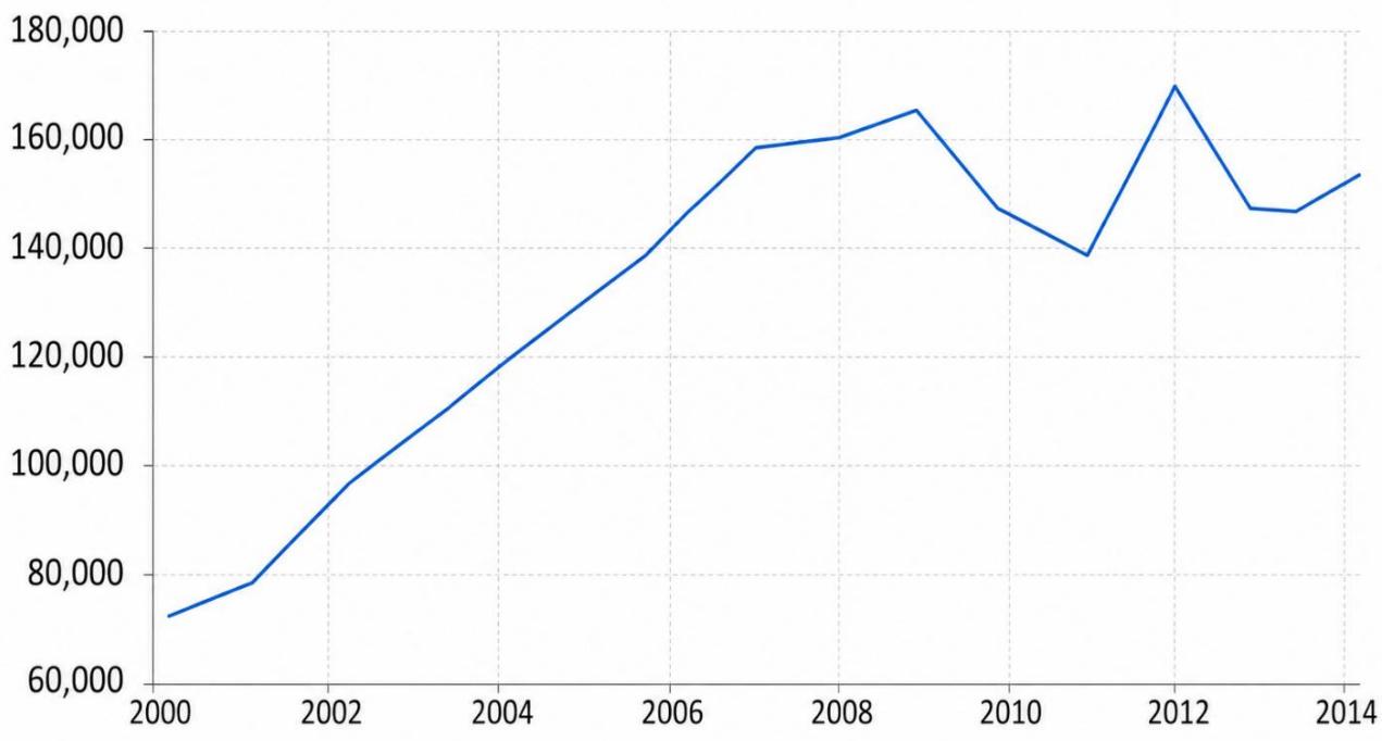
Two relevant decreases in non-financial resources take place in early 2010s (Figure 1). The first one is mainly explained by the negative settlements of the autonomous financing system corresponding to 2008 and 2009 but executed in 2010 and 2011. The second one is related to the double-dip recession also experienced by the Spanish economy in that period.
Figure 1: Non-financial resources series, 2000-2015
*In million Euros. **Source: IGAE, national accounts
Recall that the Spanish regional financing system consists of transfers to autonomous communities linked to the participation of autonomous communities in the taxes collected by the central government. The transfer is based on an estimation, which is corrected (“settled”), after two years, once collection has been definitively closed. Negative settlements, due to the mismatch between the estimated and the realized tax collection, have played a role in explaining this trend. In this context, our methodology to smooth the series becomes crucial in order to avoid such anomalies do distort the trends.
Just to complete the preliminary approach to the basic data, Table 2 shows the main descriptive statistics of the non-financial resources series. And Table 3 reports the necessary inputs to compute the public debt-to-GDP ratio across regions at the beginning of the period under scrutiny.
Table 2: Descriptive statistics of the series of non-financial resources
| Observations | Mean | Median | Std. Dev. | Minimum | Maximum | |
| Andalucía | 16 | 22,751 | 23,410 | 4,817 | 13,671 | 28,892 |
| Aragón | 16 | 3,895 | 4,166 | 1,089 | 1,575 | 5,216 |
| Baleares | 16 | 2,940 | 3,164 | 1,059 | 1,012 | 4,474 |
| Canarias | 16 | 6,794 | 7,047 | 1,113 | 4,635 | 8,234 |
| Cantabria | 16 | 1,957 | 2,121 | 525 | 851 | 2,503 |
| Castilla y León | 16 | 5,560 | 5,943 | 1,613 | 2,209 | 7,351 |
| Castilla-La Mancha | 16 | 7,679 | 8,053 | 1,806 | 3,813 | 9,786 |
| Cataluña | 16 | 21,842 | 24,109 | 5,320 | 12,545 | 29,078 |
| Comunidad de Madrid | 16 | 16,711 | 18,494 | 5,005 | 6,641 | 24,681 |
| Comunidad Foral de Navarra | 16 | 3,262 | 3,350 | 369 | 2,727 | 3,962 |
| Comunitat Valenciana | 16 | 12,503 | 13,539 | 2,734 | 7,409 | 16,162 |
| Extremadura | 16 | 3,715 | 3,992 | 976 | 1,540 | 4,741 |
| Galicia | 16 | 8,776 | 8,903 | 1,505 | 5,938 | 10,847 |
| La Rioja | 16 | 986 | 1,086 | 261 | 1,160 | 1,262 |
| País Vasco | 16 | 8,074 | 8,754 | 1,350 | 5,627 | 9,531 |
| Principado de Asturias | 16 | 3,401 | 3,632 | 891 | 1,263 | 4,403 |
| Región de Murcia | 16 | 3,683 | 4,111 | 1,047 | 1,516 | 4,847 |
| total | 16 | 134,531 | 147,174 | 30,595 | 73,405 | 172,297 |
*Ïn millions of Euros **Source: Authors from IGAE
Table 3. Debt/GDP ratio of ACs at the beginning of the simulation period.
| Debt $_{t0=2015}$ | GDP $_{t0=2015}$ | Debt $_{t0=2015}/GDP_{t0=2015}$ | |
| Andalucía | 31,643 | 144,859 | 21.8% |
| Aragón | 6,930 | 32,897 | 21.1% |
| Canarias | 6,663 | 40,596 | 16.4% |
| Cantabria | 2,677 | 12,336 | 21.7% |
| Castilla y León | 10,557 | 53,273 | 19.8% |
| Castilla-La Mancha | 13,426 | 37,138 | 36.2% |
| Cataluña | 72,675 | 204,481 | 35.5% |
| Comunidad de Madrid | 28,683 | 204,158 | 14.0% |
| Comunidad Foral de Navarra | 3,322 | 18,154 | 18.3% |
| Comunitat Valenciana | 42,003 | 100,186 | 41.9% |
| Extremadura | 3,576 | 17,916 | 20.0% |
| Galicia | 10,375 | 56,698 | 18.3% |
| Baleares | 8,330 | 28,271 | 29.5% |
| La Rioja | 1,436 | 7,967 | 18.0% |
| País Vasco | 9,486 | 65,027 | 14.6% |
| Principado de Asturias | 3,876 | 21,389 | 18.1% |
| Región de Murcia | 7,601 | 28,509 | 26.7% |
| total | 263,259 | 1,073,854 | 24.5% |
* In millions of Euros and percentage of GDP **Source: Authors, from Banco de España and INE, national accounts
The methodology for smoothing and forecasting the non-financial resources is the Holt-Winters (HW) filter. The HW methodology is a widely used exponential smoothing model in econometrics and time series analysis for modeling and forecasting data with trend and seasonality. This methodology extends the simple exponential smoothing procedures by incorporating level, trend, and seasonal components, allowing it to capture complex patterns in time series. In this subsection, we provide a concise description of the HW filter, which, as far as we know, has been hardly applied to fiscal policy topics, despite its widespread use in other areas of economics (Gardner, 2006).
The Holt–Winters method combines time-series smoothing with forecasting for future periods. In this respect, it shares similarities with ARIMA models or with regressions that use exponential or polynomial functions to fit the evolution of timeseries over time. In cross-method comparisons, the Holt–Winters approach ranks among the leading methods in terms of numerical forecasting accuracy, as measured by different indicators (Makridakis and Hibon, 2000; Makridakis et al, 2020).
This relative advantage becomes more pronounced when working with specifications that incorporate damped trends (Gardner and McKenzie, 2011), which, as will be shown below, might be our case. In any event, one of its main advantages lies in the operational simplicity with which it can be implemented in widely used software packages such as EViews or Python, and even in spreadsheet programs such as Microsoft Excel in its simpler specifications, without compromising predictive accuracy.
As noted above, the Holt–Winters method smooths the time series under analysis and, on that basis, produces forecasts for ? + ℎ periods ahead, where ? denotes the moment at which the last observation is available. In each series, three components are typically distinguished: the level, the trend, and the seasonal component. Each of these may in turn be specified in either additive or multiplicative form, depending on whether they are related through addition or multiplication. Finally, for the purpose of presenting the specification, we adopt the recurrent formulation which, in our view, simplifies the notation relative to the error-correction representation.
Our specification entails both a simplification and a complication. The simplification arises from the fact that, since we work with annual data, it is not necessary to include seasonal components in the estimation. The complication is that the multiplicative trend may well contain an additional damped-trend component, which increases the number of parameters to be estimated.
Analytically, the theoretical framework can be illustrated next3. We now focus on the specification that our data follows, as demonstrated below. Let denote the observed value of the series up to period ?. From each sample observation two elements can be extracted: (1) the level component , corresponding to a smoothing of current and past observations of , appropriately weighted according to and (2) the trend component ?, which enters multiplicatively:
\[S _ {t} = \alpha X _ {t} + (1 - \alpha) (S _ {t - 1} T _ {t - 1} ^ {\varphi})\tag{11}\]
The parameter ? reflects the weight assigned to the most recent values of the series used for forecasting, while its complement (1−?) refers to the weight attributed to earlier observations. The trend ?, which enters multiplicatively with the level in equation (11), follows the equation:
\[T _ {t} = \beta (S _ {t} / S _ {t - 1}) + (1 - \beta) (T _ {t - 1} ^ {\varphi}),\tag{12}\]
where is the parameter governing the smoothing of the trend. In particular, it determines the extent to which the trend is influenced by the immediate change in the most recent smoothed levels and , whereas weights the contribution of the trend in previous periods . The trend itself follows a damped process over time according to the parameter
At this stage of the analysis, the natural continuation of the Holt–Winters method involves searching for the parameters , and . Two main strategies exist for this purpose: minimizing the mean squared error of the differences between observed and estimated values or maximizing a log-likelihood function. We adopt the former approach.
Because we are dealing with non-linear functions, closed-form analytical solutions are difficult to obtain; therefore, numerical methods are employed. In the search for solutions, these methods do not always converge to a given proximity threshold relative to the parameter values that maximize the objective function. In this regard, the initial values used to start the iterations are often relevant. Nevertheless, after a sufficiently large number of iterations and by relaxing the convergence criterion, acceptable solutions can be obtained.
3 For further technical details on this method, see Gardner (2006) and Hyndman et al. (2008).
Once the series has been smoothed, the Holt–Winters method is completed by forecasting future values of up to period , denoted according to standard notation:
\[\widehat {X _ {t + h}} = S _ {t} T _ {t} ^ {\sum_ {i = 1} ^ {h} \varphi^ {i}}.\tag{13}\]
In our proposal, the value of the parameters such as α will play a special role, since as we have explained, this is the weight that the model gives to the most recent values of the sample. In the first simulation we consider equals 0.25, which means that we are giving relatively more weight to the past than to recent changes in the historic series of resources.
Furthermore, we will show the result of another simulation with an α equal to 0.9 as well. Determining a high α means that the projection will weigh more the most recent values of revenues. In this context, it may well imply that expenditure ceiling becomes endogenous in a sense regarding the ability of regional governments to increase their own resources and, therefore, their expenditure ceiling for the future.
In fact, something similar can be found in the LOEPSF as long changes in the computable expenditure growth are allowed if there are permanent tax collection increases/decreases. In our case, however, we introduce such possibility in the very design of the rule, so that it can influence the medium-term planning and the determination of the ceiling, not at the phasis of the compliance assessment as the current framework sets up.
In the annex, we offer details on the model specifications of the chosen alternatives for each AC, according to the AIC selection criterion and the remaining values of the specifications and projections.
6. Results
6.1. Simulation with α = 0.25, β = 0 and comparisons with the official rules.
Next, the first estimated set of values is shown. The chosen specification includes multiplicative error, multiplicative dampened trend, and obviously no seasonal term, i. e., (M, MD, N) using the standard notation. Table 4 shows two panels: the comparison of AIC criteria across different specifications and the relevant estimated parameters for that with smallest AIC, with critical statistics and technical details procedure. Convergence is achieved after only 18 iterations.
In the initial automated runs, with α equal to 0.25 and beta unrestricted, several ACs exhibited negative or unrealistically low growth projections. From a political economy standpoint, projecting a decline in non-financial revenues during a period of nominal GDP growth would not be realistic. By setting , we effectively removed the trend component that was being distorted by shortterm volatility. This transformed the model into a stable "Level-only" forecast, preventing the rule from projecting a systemic collapse in revenues that does not align with the fiscal cycle. We therefore set the value of β at 0 while α equal to 0.25.
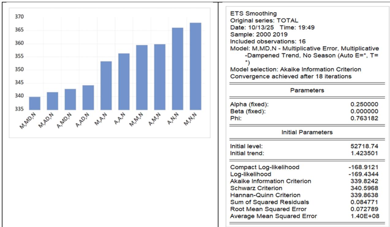
* Source: Authors
With α set at 0.25, the model adopts a "long memory" approach. This low value for α ensures that the forecast is not overly sensitive to one-off revenue spikes (noise). By combining a low α with a restricted β, we achieve a conservative but positive growth trajectory, avoiding the "downward spiral" that an unrestricted, trend-heavy model would have suggested.
The output for the total of ACs (projecting the addition of all ACs’ revenues) shows a multiplicative dampened trend (M, MD, N). Even though β is set at zero, the presence of ? parameter of 0.76 indicates that the model is designed to "moderate" or dampen any residual trend effects over time. This provides a "safety buffer", ensuring that the revenue ceiling remains grounded and does not grow at an unsustainable or explosive rate in the long run.
The fact that the trend ? equates zero does not mean that there is no trend. It means that this trend is not updated when new information is available. The trend might start at a determined value in t = 0 and it remains unchanged over time. And this is compatible with a damped parameter ? different than zero, which implies that the trend, although unaffected by new observations, is indeed slightly damped as time goes by.
Table 4: Statistics and parameters for the Holt-Winters smoothing and forecasting of total ACs non-financial resources, and AIC models selection with α = 0.25
| ETS SmoothingOriginal series: TOTALDate: 10/13/25 Time: 19:49Sample: 2000 2019Included observations: 16Model: M,MD,N - Multiplicative Error, Multiplicative -Dampened Trend, No Season (Auto E=*, T=*)Model selection: Akaike Information CriterionConvergence achieved after 18 iterations | |
| Parameters | |
| Alpha (fixed): | 0.250000 |
| Beta (fixed): | 0.000000 |
| Phi: | 0.763182 |
| Initial Parameters | |
| Initial level: | 52718.74 |
| Initial trend: | 1.423501 |
| Compact Log-likelihood | -168.9121 |
| Log-likelihood | -169.4344 |
| Akaike Information Criterion | 339.8242 |
| Schwarz Criterion | 340.5968 |
| Hannan-Quinn Criterion | 339.8638 |
| Sum of Squared Residuals | 0.084771 |
| Root Mean Squared Error | 0.072789 |
| Average Mean Squared Error | 1.40E+08 |
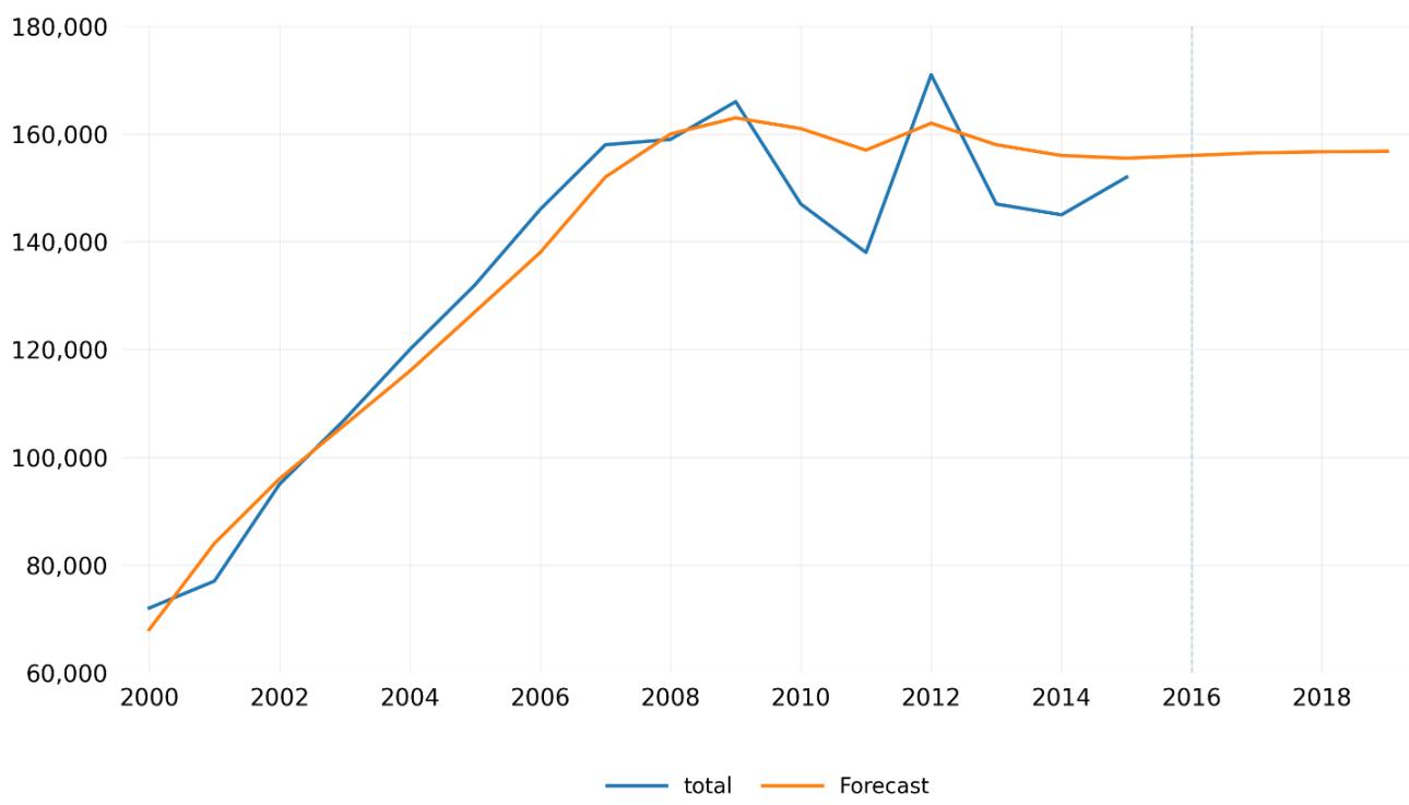
The values obtained for the estimated parameters have an immediate implication. As Figure 2 illustrates, the HW filter successfully deals with the actual data in blue, obtaining the smoothed series in orange even under the presence of pronounced peaks and valleys. But over the period 2016-2019 considered for forecasting, the slope for the projection is very flat, and the resulting rule will become significantly stringent.
Figure 2: Holt-Winters smoothing and forecasting of total ACs non-financial resources, with α = 0.25
*In millions of Euros.
Table 5. Estimation of the expenditure ceiling using expression ( 9)
| $TR_t$ , Trend Revenue ( $\alpha=0.25$ ) | Expenditure Ceiling (Proposal) | |||||||
| 2016 | 2017 | 2018 | 2019 | 2016 | 2017 | 2018 | 2019 | |
| Andalucía | 25,284 | 25,345 | 25,391 | 25,425 | 24,643 | 24,736 | 24813 | 24,876 |
| Aragón | 4,502 | 4,510 | 4,515 | 4,519 | 4,369 | 4,384 | 4396 | 4,406 |
| Canarias | 7,492 | 7,509 | 7,522 | 7,532 | 7,422 | 7,443 | 7460 | 7,473 |
| Cantabria | 2,286 | 2,291 | 2,294 | 2,296 | 2,232 | 2,240 | 2245 | 2,250 |
| Castilla y León | 8,573 | 8,584 | 8,592 | 8,598 | 8,391 | 8,412 | 8428 | 8,442 |
| Castilla-La Mancha | 6,446 | 6,459 | 6,468 | 6,475 | 6,016 | 6,051 | 6080 | 6,106 |
| Cataluña | 26,945 | 27,188 | 27,390 | 27,559 | 24,640 | 24,998 | 25310 | 25,583 |
| Comunidad de Madrid | 20,961 | 21,044 | 21,106 | 21,152 | 20,854 | 20,942 | 21009 | 21,061 |
| Comunidad Foral de Navarra | 3,496 | 3,505 | 3,513 | 3,520 | 3,447 | 3,459 | 3470 | 3,478 |
| Comunitat Valenciana | 14,761 | 14,836 | 14,896 | 14,944 | 13,312 | 13,460 | 13588 | 13,701 |
| Extremadura | 4,213 | 4,215 | 4,217 | 4,218 | 4,151 | 4,156 | 4161 | 4,164 |
| Galicia | 9,580 | 9,602 | 9,618 | 9,631 | 9,430 | 9,459 | 9483 | 9,502 |
| Baleares | 4,123 | 4,162 | 4,193 | 4,218 | 3,890 | 3,941 | 3983 | 4,019 |
| La Rioja | 1,167 | 1,170 | 1,171 | 1,172 | 1,147 | 1,151 | 1153 | 1,155 |
| País Vasco | 9,362 | 9,412 | 9,453 | 9,487 | 9,310 | 9,363 | 9407 | 9,443 |
| Principado de Asturias | 3,853 | 3,855 | 3,857 | 3,858 | 3,798 | 3,803 | 3808 | 3,811 |
| Región de Murcia | 4,377 | 4,387 | 4,394 | 4,400 | 4,182 | 4,202 | 4219 | 4,233 |
| total | 157,420 | 158,074 | 158,592 | 159,004 | 151,237 | 152,200 | 153012 | 153,703 |
*In Millions of Euros **Source: Authors
Anyway, Table 5 shows the spending ceilings resulting from the application of expression ( 9) for the period 2016-2019, taking as basis the parameters obtained for the smoothed series of trend revenues. From these spending ceilings4, the resulting reference growth rate can be calculated and compared with the officially established rate (Table 6). The comparison shows that the growth rates of spending under the proposal are much more stringent than the official rates, as we could deduct from the (almost null) slope of the smoothed trend of revenues.
4 The figure for total in this Table 5 is the addition of the trend revenues and the expenditure ceilings of individual ACs, not the projection of the total ACs revenues, that can be seen in Figure 2 and Table 4 above, and its corresponding ceiling.
Table 6. Difference in percentage in expenditure growth allowed by the proposal, the growth reference rate at official expenditure rule and the computable spending growth, used to assess compliance with the rule.
| Expenditure Growth according to proposal | Official ER Rate | Computable spending growth | |||||||
| 2017 | 2018 | 2019 | 2017 | 2018 | 2019 | 2017 | 2018 | 2019 | |
| Andalucía | 0.4 | 0.3 | 0.3 | 2.1 | 2.4 | 2.7 | 2.8 | 4.9 | 1.5 |
| Aragón | 0.3 | 0.3 | 0.2 | 2.1 | 2.4 | 2.7 | 3.9 | 1.7 | 4.4 |
| Canarias | 0.3 | 0.2 | 0.2 | 2.1 | 2.4 | 2.7 | 4.4 | 4.5 | 3.4 |
| Cantabria | 0.3 | 0.3 | 0.2 | 2.1 | 2.4 | 2.7 | 0.6 | 2.7 | 6.9 |
| Castilla y León | 0.2 | 0.2 | 0.2 | 2.1 | 2.4 | 2.7 | 5.2 | -1.6 | 4.5 |
| Castilla-La Mancha | 0.6 | 0.5 | 0.4 | 2.1 | 2.4 | 2.7 | 4.0 | 1.5 | 8.6 |
| Cataluña | 1.5 | 1.2 | 1.1 | 2.1 | 2.4 | 2.7 | 3.8 | 1.7 | 6.3 |
| Comunidad de Madrid | 0.4 | 0.3 | 0.2 | 2.1 | 2.4 | 2.7 | 5.3 | 1.9 | 6.3 |
| Comunidad Foral de Navarra | 0.3 | 0.3 | 0.2 | 2.1 | 2.4 | 2.7 | 10.9 | 3.2 | 4.2 |
| Comunitat Valenciana | 1.1 | 1.0 | 0.8 | 2.1 | 2.4 | 2.7 | 3.2 | 7.8 | 6.8 |
| Extremadura | 0.1 | 0.1 | 0.1 | 2.1 | 2.4 | 2.7 | 0.1 | -2.3 | 7.2 |
| Galicia | 0.3 | 0.2 | 0.2 | 2.1 | 2.4 | 2.7 | 2.1 | 1.2 | 6.0 |
| Baleares | 1.3 | 1.1 | 0.9 | 2.1 | 2.4 | 2.7 | 2.7 | 11.9 | 2.2 |
| La Rioja | 0.3 | 0.2 | 0.2 | 2.1 | 2.4 | 2.7 | 4.1 | 3.0 | 1.7 |
| País Vasco | 0.6 | 0.5 | 0.4 | 2.1 | 2.4 | 2.7 | 2.9 | 0.4 | 4.2 |
| Principado de Asturias | 0.1 | 0.1 | 0.1 | 2.1 | 2.4 | 2.7 | 1.8 | 1.1 | 6.3 |
| Región de Murcia | 0.5 | 0.4 | 0.3 | 2.1 | 2.4 | 2.7 | 3.4 | 3.0 | 6.5 |
| total | 0.6 | 0.5 | 0.5 | 2.1 | 2.4 | 2.7 | 3.6 | 2.8 | 5.1 |
*Source: authors and compliance reports[1] **The figures for computable spending in year 2017 changed from the report published in October 2018 to the report published in October 2019. The latter has been used. [1] https://www.hacienda.gob.es/es-ES/CDI/Paginas/EstabilidadPresupuestaria/InformesCompletosLEP.aspx
Apart from the stringency of the rule, the fact that the forecast is not giving more weight to recent developments in the revenue side means that policymakers will not be incentivized to increase them, since it will have hardly impact on their future spending. This is why we think the parameter α should be substantially higher.
Another justification for increasing the value of parameter α is to ensure the smoothed series remains "responsive" to the current economic reality. When α is low, the smoothed series lags significantly behind the real series, which can lead to a misreading of the output gap or the structural fiscal position. During a recession the real series drops. Because the smoothed series incorporates past higher values, it stays above the real series. In a fiscal context, this is "countercyclical" as it suggests that the drop is temporary and prevents an immediate, drastic cut in spending that would further damage the economy. During expansion the real series rises. The smoothed series, even with a high α, will initially stay below the real series.
This gap is what forces the "countercyclical" behavior by keeping the fiscal reference below the actual peak of the expansion, preventing the government from spending temporary revenue windfalls. By choosing α = 0.9, the model is calibrated to push the "smoothed" line to follow the real series more closely than a lower α would, ensuring that the fiscal rule adapts almost instantly to a new structural level after a recession or expansion has consolidated.
Since the gap with the actual revenue in the most recent years will be lower in the high α case, the countercyclical properties would be lower in the case of a high α than in the case of a low α, even if it reflects better possible structural changes in the revenue level, the output gap and/or the structural fiscal position. To illustrate this case, next we change the specification to α = 0.9, which involves more weight to the most recent observation when estimating the parameters.
6.2 Simulation with α = 0.9 and comparison with the official rules
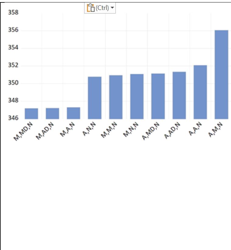
Next, we present in Table 7 the specific values of the estimation and according to the AIC criterion for the total of the ACs. In this case, we will not set the value of since in most cases, the projection yields a positive slope. In cases that it does not produce a positive slope, we will impose the additional restriction of positive growth, when choosing the model through the AIC criterion5.
The selected specification, if we look at the projection of the total of ACs’ revenues, is again multiplicative error, multiplicative dampened trend, and no seasonality. Convergence is quicky achieved, with a dumped parameter (0.82) relatively close to the previous one (0.76), and again a null value for the parameter of the trend, even if in this case, we did not impose any value to the parameter
5 When estimating the individual ceiling for each AC, we have considered an additional restriction of positive growth, apart from the AIC criterion, to choose the smoothing and projection model. Depending on the growth of the revenue at the end of the series considered, some ACs would have a zero or even negative growth projection, if only the AIC criterion would have been considered, and, as explained above, we believe that such a stringency would be difficult to accept from a political economy point of view. This is the case of Galicia, where the AIC criterion would have produced a 0-growth trend with the model (M, N, N) (Multiplicative Error, No Trend, No Season), the best model according to the AIC criterion. Instead, we chose the (M, AD, N) (Multiplicative Error, Additive-Dampened Trend, No Season) model, the third best model according to the AIC criterion, which implied positive growth. The same applies to Región de Murcia, where the second-best model according to the AIC criterion was chosen and Comunidad Foral de Navarra, where the sixth-best model according to the AIC criterion was chosen. See Annex II.
Table 7: Statistics and parameters for the Holt-Winters smoothing and forecasting of total ACs non-financial resources with α = 0.9.
| Parameters | |
| Alpha (fixed): | 0.900000 |
| Beta: | 0.000000 |
| Phi: | 0.824161 |
| Initial Parameters | |
| Initial level: | 59893.21 |
| Initial trend: | 1.259092 |
| Compact Log-likelihood | -170.5880 |
| Log-likelihood | -171.1103 |
| Akaike Information Criterion | 347.1760 |
| Schwarz Criterion | 349.4938 |
| Hannan-Quinn Criterion | 347.2947 |
| Sum of Squared Residuals | 0.105300 |
| Root Mean Squared Error | 0.081125 |
| Average Mean Squared Error | 1.89E+08 |
Figure 3: Holt-Winters smoothing and forecasting of total ACs non-financial resources, with α = 0.9
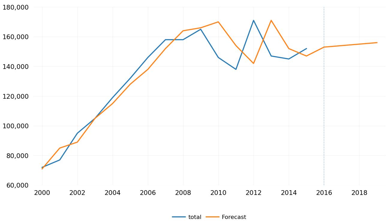
*In millions of Euros **Source: Authors
Figure 3 already points to a ceiling with more slope than in the previous case, even if the smoothing is not so effective to attenuate the peaks. This more intense slope can be seen both in periods regarding actual data and in the years subject to future projection. This latter fact is due to the remarkable increase in revenues in the last year of sample, which has been more weighted than in the previous simulation. We also show in Table 8 the estimated trend revenue and the corresponding ceiling in this expenditure rule, according to expression6 ( 9).
6 Again, the figure for total in this Table 8 is the addition of the trend revenues and the expenditure ceilings of individual ACs, not the projection of the total ACs revenues, that can be seen in Figure 3 and Table 7 above, and its corresponding ceiling.
Table 8: Estimation of the expenditure ceiling using expression ( 9)
| TRt, Trend Revenue (α=09) | Expenditure ceiling proposal | |||||||
| 2016 | 2017 | 2018 | 2019 | 2016 | 2017 | 2018 | 2019 | |
| Andalucía | 25,423 | 26,588 | 27,753 | 28,917 | 24,782 | 25,979 | 27,175 | 28,368 |
| Aragón | 4,350 | 4,407 | 4,456 | 4,498 | 4,217 | 4,281 | 4,336 | 4,384 |
| Canarias | 7,568 | 7,614 | 7,652 | 7,683 | 7,499 | 7,548 | 7,589 | 7,624 |
| Cantabria | 2,236 | 2,249 | 2,259 | 2,267 | 2,182 | 2,198 | 2,211 | 2,221 |
| Castilla y León | 8,256 | 8,291 | 8,319 | 8,340 | 8,074 | 8,119 | 8,155 | 8,184 |
| Castilla-La Mancha | 6,111 | 6,203 | 6,283 | 6,352 | 5,681 | 5,795 | 5,895 | 5,983 |
| Cataluña | 26,942 | 28,123 | 29,303 | 30,483 | 24,638 | 25,933 | 27,223 | 28,507 |
| Comunidad de Madrid | 20,835 | 21,201 | 21,523 | 21,806 | 20,728 | 21,099 | 21,426 | 21,714 |
| Comunidad Foral de Navarra | 3,543 | 3,570 | 3,594 | 3,615 | 3,495 | 3,524 | 3,550 | 3,574 |
| Comunitat Valenciana | 15,141 | 15,833 | 16,525 | 17,216 | 13,692 | 14,456 | 15,217 | 15,974 |
| Extremadura | 4,114 | 4,133 | 4,149 | 4,161 | 4,052 | 4,074 | 4,092 | 4,107 |
| Galicia | 9,444 | 9,555 | 9,654 | 9,743 | 9,294 | 9,412 | 9,519 | 9,614 |
| Baleares | 4,634 | 4,946 | 5,258 | 5,571 | 4,401 | 4,725 | 5,048 | 5,371 |
| La Rioja | 1,171 | 1,185 | 1,196 | 1,206 | 1,151 | 1,166 | 1,178 | 1,188 |
| País Vasco | 9,726 | 10,034 | 10,342 | 10,650 | 9,674 | 9,985 | 10,296 | 10,606 |
| Principado de Asturias | 3,687 | 3,691 | 3,694 | 3,696 | 3,632 | 3,639 | 3,645 | 3,649 |
| Región de Murcia | 4,359 | 4,435 | 4,501 | 4,559 | 4,165 | 4,250 | 4,325 | 4,392 |
| total | 157,542 | 162,058 | 166,459 | 170,762 | 151,359 | 156,184 | 160,879 | 165,461 |
*figures in millions of euros **Source: Authors
Again, for sake of comparison, we report in Table 9 the growth rates of expenditure according to our proposed ceiling, the official rates in the expenditure rule and the computable spending used to assess compliance.
Table 9: Expenditure growth rates with proposal against official expenditure rule, in percentage
| Expenditure Growth according to proposal | Official ER Rate | Computable spending* growth | |||||||
| 2017 | 2018 | 2019 | 2017 | 2018 | 2019 | 2017 | 2018 | 2019 | |
| Andalucía | 4.8 | 4.6 | 4.4 | 2.1 | 2.4 | 2.7 | 2.8 | 4.9 | 1.5 |
| Aragón | 1.5 | 1.3 | 1.1 | 2.1 | 2.4 | 2.7 | 3.9 | 1.7 | 4.4 |
| Canarias | 0.7 | 0.5 | 0.5 | 2.1 | 2.4 | 2.7 | 4.4 | 4.5 | 3.4 |
| Cantabria | 0.7 | 0.6 | 0.5 | 2.1 | 2.4 | 2.7 | 0.6 | 2.7 | 6.9 |
| Castilla y León | 0.6 | 0.4 | 0.4 | 2.1 | 2.4 | 2.7 | 5.2 | -1.6 | 4.5 |
| Castilla-La Mancha | 2.0 | 1.7 | 1.5 | 2.1 | 2.4 | 2.7 | 4.0 | 1.5 | 8.6 |
| Cataluña | 5.3 | 5.0 | 4.7 | 2.1 | 2.4 | 2.7 | 3.8 | 1.7 | 6.3 |
| Comunidad de Madrid | 1.8 | 1.5 | 1.3 | 2.1 | 2.4 | 2.7 | 5.3 | 1.9 | 6.3 |
| Comunidad Foral de Navarra | 0.8 | 0.7 | 0.7 | 2.1 | 2.4 | 2.7 | 10.9 | 3.2 | 4.2 |
| Comunitat Valenciana | 5.6 | 5.3 | 5.0 | 2.1 | 2.4 | 2.7 | 3.2 | 7.8 | 6.8 |
| Extremadura | 0.6 | 0.4 | 0.4 | 2.1 | 2.4 | 2.7 | 0.1 | -2.3 | 7.2 |
| Galicia | 1.3 | 1.1 | 1.0 | 2.1 | 2.4 | 2.7 | 2.1 | 1.2 | 6.0 |
| Baleares | 7.4 | 6.8 | 6.4 | 2.1 | 2.4 | 2.7 | 2.7 | 11.9 | 2.2 |
| La Rioja | 1.2 | 1.1 | 0.9 | 2.1 | 2.4 | 2.7 | 4.1 | 3.0 | 1.7 |
| País Vasco | 3.2 | 3.1 | 3.0 | 2.1 | 2.4 | 2.7 | 2.9 | 0.4 | 4.2 |
| Principado de Asturias | 0.2 | 0.2 | 0.1 | 2.1 | 2.4 | 2.7 | 1.8 | 1.1 | 6.3 |
| Región de Murcia | 2.0 | 1.8 | 1.5 | 2.1 | 2.4 | 2.7 | 3.4 | 3.0 | 6.5 |
| total | 3.2 | 3.0 | 2.8 | 2.1 | 2.4 | 2.7 | 3.6 | 2.8 | 5.1 |
*The figures for computable spending in year 2017 changed from the report published in October 2018 to the report published in October 2019. The latter has been used.
Table 9 shows how the growth rates of expenditure allowed by the rule are higher with this specification and generally higher than the official reference rate. This is due to the increasing revenues in the year previous to the period considered, which is determinant when α is relatively high. Focusing on the growth rates, we conclude that this rule is more permissive than the official one. However, if we compare the resulting ceiling of this rule with the expenditure effectively incurred in these years we check that, in general, the ceiling would have been breached by ACs in this period7.
7 We use the non-financial spending from national accounts as the expenditure effectively incurred, since this is the measure to calculate the deficit. The data can be accessed from this link: https://www.igae.pap.hacienda.gob.es/sitios/igae/es-
ES/Contabilidad/ContabilidadNacional/Publicaciones/Paginas/ianofinancierasCA.aspx
Table 10. Difference between ceiling according to proposal and actual expenditure
| Expenditure ceiling according to proposal | Actual Expenditure (Non-financial uses) | Difference | ||||||||||
| 2016 | 2017 | 2018 | 2019 | 2016 | 2017 | 2018 | 2019 | 2016 | 2017 | 2018 | 2019 | |
| Andalucía | 24,782 | 25,979 | 27,175 | 28,368 | 25,655 | 26,323 | 27,839 | 28,654 | -3.4% | -1.3% | -2.4% | -1.0% |
| Aragón | 4,217 | 4,281 | 4,336 | 4,384 | 4,897 | 5,095 | 5,290 | 5,487 | -13.9% | -16.0% | -18.0% | -20.1% |
| Canarias | 7,499 | 7,548 | 7,589 | 7,624 | 7,989 | 8,276 | 8,791 | 9,291 | -6.1% | -8.8% | -13.7% | -17.9% |
| Cantabria | 2,182 | 2,198 | 2,211 | 2,221 | 2,382 | 2,411 | 2,525 | 2,674 | -8.4% | -8.8% | -12.4% | -16.9% |
| Castilla y León | 8,074 | 8,119 | 8,155 | 8,184 | 8,638 | 8,991 | 8,992 | 9,789 | -6.5% | -9.7% | -9.3% | -16.4% |
| Castilla-La Mancha | 5,681 | 5,795 | 5,895 | 5,983 | 6,346 | 6,635 | 6,948 | 7,477 | -10.5% | -12.7% | -15.2% | -20.0% |
| Cataluña | 24,638 | 25,933 | 27,223 | 28,507 | 29,817 | 30,852 | 32,141 | 34,409 | -17.4% | -15.9% | -15.3% | -17.2% |
| Comunidad de Madrid | 20,728 | 21,099 | 21,426 | 21,714 | 23,845 | 25,348 | 26,380 | 27,815 | -13.1% | -16.8% | -18.8% | -21.9% |
| Comunidad Foral de Navarra | 3,495 | 3,524 | 3,550 | 3,574 | 3,757 | 3,697 | 4,040 | 4,285 | -7.0% | -4.7% | -12.1% | -16.6% |
| Comunitat Valenciana | 13,692 | 14,456 | 15,217 | 15,974 | 17,057 | 17,345 | 18,886 | 19,998 | -19.7% | -16.7% | -19.4% | -20.1% |
| Extremadura | 4,052 | 4,074 | 4,092 | 4,107 | 4,342 | 4,382 | 4,491 | 4,719 | -6.7% | -7.0% | -8.9% | -13.0% |
| Galicia | 9,294 | 9,412 | 9,519 | 9,614 | 9,547 | 9,732 | 10,014 | 10,678 | -2.6% | -3.3% | -4.9% | -10.0% |
| Baleares | 4,401 | 4,725 | 5,048 | 5,371 | 4,662 | 4,776 | 5,448 | 5,666 | -5.6% | -1.1% | -7.3% | -5.2% |
| La Rioja | 1,151 | 1,166 | 1,178 | 1,188 | 1,217 | 1,266 | 1,322 | 1,392 | -5.4% | -7.9% | -10.9% | -14.6% |
| País Vasco | 9,674 | 9,985 | 10,296 | 10,606 | 10,127 | 10,358 | 10,541 | 11,060 | -4.5% | -3.6% | -2.3% | -4.1% |
| Principado de Asturias | 3,632 | 3,639 | 3,645 | 3,649 | 3,870 | 3,947 | 4,078 | 4,295 | -6.1% | -7.8% | -10.6% | -15.0% |
| Región de Murcia | 4,165 | 4,250 | 4,325 | 4,392 | 5,008 | 5,149 | 5,369 | 5,708 | -16.8% | -17.5% | -19.4% | -23.1% |
| total | 151,359 | 156,184 | 160,879 | 165,461 | 169,078 | 174,520 | 183,022 | 193,331 | -10.5% | -10.5% | -12.1% | -14.4% |
ource: authors and IG illions of euros and perc
Table 10 shows this. The average distance with respect to the actual expenditure is about 12 percent lower in the proposal. The actual expenditure is higher in all cases (the negative figures in the column headed by “Difference”) than the expenditure allowed by the ceiling determined by the proposal, in some cases (Region de Murcia) in percentages amounting to 23 percent. Some AC would have been close to complying with this ceiling in some year (Andalucía), but in general, all seem to be far from compliance.
The reason for this result, apart from the fact that this rule aims at debt reduction, is that we are considering a period of economic recovery, with positive output gaps, and where official targets in terms of public deficits were pro-cyclical. It led to expenditure trajectories well above those of revenue. The rule proposed here, by contrast, aims at reaching a fiscal balance in the medium term, so that it would have been more restrictive.
The apparent stringency of the rule would be nuanced, however, if we were to compare the ceiling proposed by the rule with the “computable spending” as appears in the compliance reports8. For this exercise we are comparing the “computable spending”, as it appears in the compliance reports, with the expenditure ceilings in the proposal9.
8 In order to calculate the computable spending, the following concepts are subtracted from the non-financial expenditures in national accounts: interest payments, expenditures financed by the EU, expenditures financed by other public administrations, transfers to the State under the Financing System, transfers to Local Governments under the Financing System, and regulatory changes with permanent revenue increases.
9 https://www.hacienda.gob.es/es-ES/CDI/Paginas/EstabilidadPresupuestaria/InformesCompletosLEP.aspx
ference ceiling and computable expenditure at the comp Authors and Ministry of Finance (complianc
| Ceiling according to proposal | Computable expenditure at official ER | Difference | ||||||||||
| 2016 | 2017 | 2018 | 2019 | 2016 | 2017 | 2018 | 2019 | 2016 | 2017 | 2018 | 2019 | |
| Andalucía | 24,782 | 25,979 | 27,175 | 28,368 | 22,046 | 22,666 | 23,780 | 24,145 | 11.0% | 12.8% | 12.5% | 14.9% |
| Aragón | 4,217 | 4,281 | 4,336 | 4,384 | 4,256 | 4,422 | 4,498 | 4,697 | -0.9% | -3.3% | -3.7% | -7.1% |
| Canarias | 7,499 | 7,548 | 7,589 | 7,624 | 5,959 | 6,220 | 6,499 | 6,717 | 20.5% | 17.6% | 14.4% | 11.9% |
| Cantabria | 2,182 | 2,198 | 2,211 | 2,221 | 2,120 | 2,133 | 2,190 | 2,341 | 2.8% | 3.0% | 0.9% | -5.4% |
| Castilla y León | 8,074 | 8,119 | 8,155 | 8,184 | 7,566 | 7,962 | 7,838 | 8,194 | 6.3% | 1.9% | 3.9% | -0.1% |
| Castilla-La Mancha | 5,681 | 5,795 | 5,895 | 5,983 | 5,474 | 5,693 | 5,778 | 6,274 | 3.7% | 1.8% | 2.0% | -4.9% |
| Cataluña | 24,638 | 25,933 | 27,223 | 28,507 | 25,021 | 25,962 | 26,393 | 28,057 | -1.6% | -0.1% | 3.0% | 1.6% |
| Comunidad de Madrid | 20,728 | 21,099 | 21,426 | 21,714 | 17,388 | 18,316 | 18,669 | 19,843 | 16.1% | 13.2% | 12.9% | 8.6% |
| Comunidad Foral de Navarra | 3,495 | 3,524 | 3,550 | 3,574 | 2,634 | 2,921 | 3,015 | 3,141 | 24.6% | 17.1% | 15.1% | 12.1% |
| Comunitat Valenciana | 13,692 | 14,456 | 15,217 | 15,974 | 13,860 | 14,307 | 15,420 | 16,470 | -1.2% | 1.0% | -1.3% | -3.1% |
| Extremadura | 4,052 | 4,074 | 4,092 | 4,107 | 3,731 | 3,736 | 3,649 | 3,911 | 7.9% | 8.3% | 10.8% | 4.8% |
| Galicia | 9,294 | 9,412 | 9,519 | 9,614 | 8,239 | 8,410 | 8,514 | 9,024 | 11.4% | 10.7% | 10.6% | 6.1% |
| Baleares | 4,401 | 4,725 | 5,048 | 5,371 | 3,108 | 3,191 | 3,571 | 3,648 | 29.4% | 32.5% | 29.3% | 32.1% |
| La Rioja | 1,151 | 1,166 | 1,178 | 1,188 | 1,136 | 1,183 | 1,219 | 1,240 | 1.3% | -1.5% | -3.5% | -4.3% |
| País Vasco | 9,674 | 9,985 | 10,296 | 10,606 | 9,544 | 9,818 | 9,854 | 10,264 | 1.3% | 1.7% | 4.3% | 3.2% |
| Principado de Asturias | 3,632 | 3,639 | 3,645 | 3,649 | 3,455 | 3,517 | 3,556 | 3,779 | 4.9% | 3.4% | 2.4% | -3.6% |
| Región de Murcia | 4,165 | 4,250 | 4,325 | 4,392 | 4,250 | 4,395 | 4,526 | 4,822 | -2.0% | -3.4% | -4.6% | -9.8% |
| total | 151,359 | 156,184 | 160,879 | 165,461 | 139,709 | 144,789 | 148,896 | 156,501 | 7.7% | 7.3% | 7.4% | 5.4% |
According to Table 11, the total computable spending is on average around 7 percent lower than the expenditure ceiling in the proposal, with most of the ACs having a lower expenditure than the one determined by the proposed rule. In any case, this comparison is included only for reference purposes, since these magnitudes should not be directly compared. The computable expenditure is calculated in the official rule in order to assess compliance whether it is lower than the reference rate. But in our proposal, compliance is measured by reference to an expenditure ceiling that determines the limit of the Non-Financial Uses (NFUs) in public spending over the period.
In Figure 4 we compare the ceiling according to the proposal, the NFUs, the computable spending, the if it had grown according to the official ER, and the computable spending growing at the official ER. This figure illustrates the stringency of the proposed ceiling even if the growth is similar or higher than the official rule. It also illustrates that the total expenditure, without adjustments related to the computable spending, was well above the growth determined by the official rule. One possible reason is the consolidation of non-compliance with the current rule.
Figure 4: Expenditure ceiling according to the proposal, non-financial uses, computable spending, NFU growing at official ER and computable spending growing at official ER
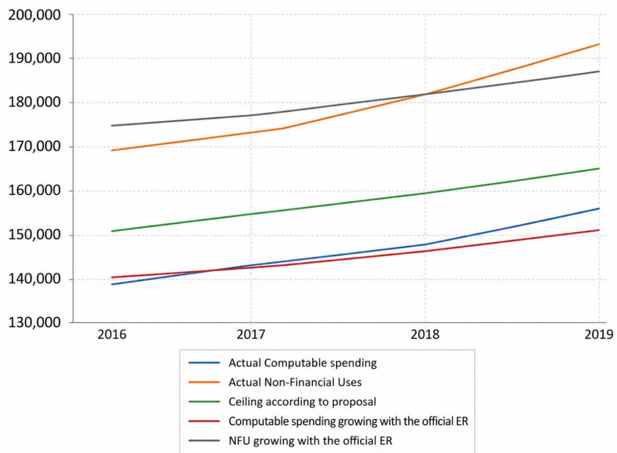
*In millions of Euros **Authors’ computations and compliance reports
According to the LOEPSF, once the expenditure rule is breached the AC should submit a PEF, but this does not guarantee the return to the allowed expenditure trend. In fact, we see that the growth of computable spending was well above the growth determined by the rule in compliance at the end of the period. In contrast with the official methodology of application of the rule, based on estimating the computable spending for the next year applying the reference rate to the settled expenditure, irrespective of compliance with the rule, our proposal is a ceiling pre-determined for the 4 years period, remaining in place irrespective of a punctual yearly non-compliance.
In what follows, we compare the fiscal outcome in terms of deficit or surplus in case of exact compliance with the ceiling determined by the proposed rule and considering the actual nonfinancial resources with the official deficit target set by the government. We are assuming the total revenues are completely exogenous to the level of public expenditure and equal to those that were collected.
Table 12: Fiscal outcome if strict compliance with the proposed fiscal rule vs official deficit target, in percentage of GDP
| fiscal balance if strict compliance with the ceiling | Official deficit targets | |||||||
| 2016 | 2017 | 2018 | 2019 | 2016 | 2017 | 2018 | 2019 | |
| Andalucía | 0.0 | -0.1 | -0.1 | -0.2 | -0.7 | -0.6 | -0.4 | -0.1 |
| Aragón | 0.8 | 1.3 | 2.2 | 1.9 | -0.7 | -0.6 | -0.4 | -0.1 |
| Canarias | 0.9 | 2.3 | 4.7 | 4.2 | -0.7 | -0.6 | -0.4 | -0.1 |
| Cantabria | 0.1 | 1.2 | 2.0 | 2.2 | -0.7 | -0.6 | -0.4 | -0.1 |
| Castilla y León | 0.3 | 0.5 | 1.2 | 1.7 | -0.7 | -0.6 | -0.4 | -0.1 |
| Castilla-La Mancha | 0.9 | 1.4 | 2.2 | 2.3 | -0.7 | -0.6 | -0.4 | -0.1 |
| Cataluña | 1.5 | 1.7 | 1.7 | 1.8 | -0.7 | -0.6 | -0.4 | -0.1 |
| Comunidad de Madrid | 0.8 | 1.4 | 1.9 | 2.3 | -0.7 | -0.6 | -0.4 | -0.1 |
| Comunidad Foral de Navarra | 0.6 | 2.1 | 2.9 | 3.8 | -0.7 | -0.6 | -0.4 | -0.1 |
| Comunitat Valenciana | 1.7 | 1.9 | 1.9 | 1.5 | -0.7 | -0.6 | -0.4 | -0.1 |
| Extremadura | -0.1 | 0.7 | 1.7 | 1.8 | -0.7 | -0.6 | -0.4 | -0.1 |
| Galicia | -0.1 | 0.3 | 1.0 | 1.2 | -0.7 | -0.6 | -0.4 | -0.1 |
| Baleares | 0.3 | 0.4 | 0.8 | 0.3 | -0.7 | -0.6 | -0.4 | -0.1 |
| La Rioja | 0.3 | 0.9 | 1.4 | 1.9 | -0.7 | -0.6 | -0.4 | -0.1 |
| País Vasco | 0.0 | 2.1 | 1.1 | 1.1 | -0.7 | -0.6 | -0.4 | -0.1 |
| Principado de Asturias | 0.6 | 1.0 | 1.9 | 2.0 | -0.7 | -0.6 | -0.4 | -0.1 |
| Región de Murcia | 1.1 | 1.5 | 2.0 | 2.3 | -0.7 | -0.6 | -0.4 | -0.1 |
| total | 0.7 | 1.2 | 1.6 | 1.7 | -0.7 | -0.6 | -0.4 | -0.1 |
Source: authors and compliance reports
As expected, Table 12 shows that the fiscal outcome if AC were to comply with the proposed rule would have been such that it would have made them comply with the official deficit targets. Per construction, the movements of revenues above their trend are explaining this surplus outcome, in a period where revenues were recovering and even growing above the trend at the middle of the period concerned. These movements could give ACs extra fiscal space that could be used to build a buffer, as the theory prescribes, for the case of expenditure rules. This buffer could be used to have extra spending in times when actual revenue grows below its trend. Or it could be used to increase investment expenditure or even to reduce further the debt stock. All in all, what can be seen in Table 12 is a remarkable anti-cyclical behavior of the rule proposed as long as positive fiscal balances are generated across expansionary periods.
Table 13 shows now that an important feature of this rule is that it ensures a predetermined path of debt reduction, irrespective of the business cycle. We compare the debt reduction that could have been achieved through the second part of the expression (9), with the actual evolution of debt in this period. In the period concerned the stock of debt merely decreased by 0.8 percent of the GDP at the aggregate level, which is merely 3.4 percentual points of the initial stock, in the four years considered.
Table 13: Actual debt reduction observed, in percentage
| Debt/GDP in 2015 | 2016 | 2017 | 2018 | 2019 | total | in percentage of initial debt/GDP | |
| Andalucía | 21.8 | 22.5 | 22.0 | 22.1 | 21.5 | -0.4 | -1.7 |
| Aragón | 21.1 | 21.9 | 22.3 | 22.4 | 21.9 | 0.8 | 3.7 |
| Canarias | 16.4 | 16.5 | 15.9 | 14.9 | 14.0 | -2.4 | -14.6 |
| Cantabria | 21.7 | 22.7 | 22.9 | 23.1 | 22.5 | 0.8 | 3.6 |
| Castilla y León | 19.8 | 20.7 | 21.2 | 21.1 | 20.9 | 1.0 | 5.3 |
| Castilla-La Mancha | 36.2 | 36.7 | 36.2 | 35.5 | 35.3 | -0.9 | -2.5 |
| Cataluña | 35.5 | 35.3 | 35.1 | 34.4 | 33.2 | -2.4 | -6.7 |
| Comunidad de Madrid | 14.0 | 14.3 | 14.7 | 14.5 | 13.8 | -0.2 | -1.6 |
| Comunidad Foral de Navarra | 18.3 | 18.5 | 18.6 | 17.2 | 15.8 | -2.5 | -13.7 |
| Comunitat Valenciana | 41.9 | 43.3 | 42.8 | 42.1 | 41.9 | 0.0 | -0.1 |
| Extremadura | 20.0 | 21.9 | 22.5 | 23.0 | 23.1 | 3.1 | 15.5 |
| Galicia | 18.3 | 18.6 | 18.6 | 18.2 | 17.6 | -0.7 | -3.7 |
| Baleares | 29.5 | 28.7 | 28.1 | 26.6 | 26.1 | -3.3 | -11.4 |
| La Rioja | 18.0 | 18.6 | 18.9 | 18.5 | 18.2 | 0.2 | 1.1 |
| País Vasco | 14.6 | 14.8 | 14.6 | 14.0 | 12.7 | -1.9 | -12.8 |
| Principado de Asturias | 18.1 | 18.9 | 18.8 | 18.7 | 18.4 | 0.3 | 1.4 |
| Región de Murcia | 26.7 | 28.3 | 28.8 | 29.7 | 29.6 | 2.9 | 11.0 |
| total | 24.5 | 24.9 | 24.8 | 24.4 | 23.7 | -0.8 | -3.4 |
*In percentage of the GDP and percentual change **Source: Banco de España
In contrast, Table 14 shows that with the proposed rule ACs would have generated enough fiscal space to reduce their debt by 5.2 points of the GDP, which is around a fifth of their initial debt stock, in those 4 years. The proposed rule would have imposed a higher debt reduction to those ACs with a higher stock of debt (Comunitat Valenciana, Cataluña, Baleares, Castilla-La Mancha).
Table 14. Debt reduction according to proposal, in percentage
| Debt/GDP in 2015 | 2016 | 2017 | 2018 | 2019 | total | in percentage of initial debt/GDP | |
| Andalucía | 21.8 | 20.9 | 19.6 | 18.6 | 17.7 | -4.1 | -18.8 |
| Aragón | 21.1 | 19.9 | 18.7 | 17.8 | 16.9 | -4.1 | -19.7 |
| Canarias | 16.4 | 15.7 | 14.8 | 14.1 | 13.6 | -2.8 | -17.3 |
| Cantabria | 21.7 | 20.6 | 19.4 | 18.4 | 17.5 | -4.2 | -19.5 |
| Castilla y León | 19.8 | 18.9 | 18.2 | 17.1 | 16.5 | -3.3 | -16.6 |
| Castilla-La Mancha | 36.2 | 33.9 | 31.6 | 29.4 | 27.9 | -8.2 | -22.8 |
| Cataluña | 35.5 | 33.1 | 30.8 | 28.9 | 26.9 | -8.6 | -24.3 |
| Comunidad de Madrid | 14.0 | 13.5 | 12.8 | 12.3 | 11.7 | -2.4 | -16.8 |
| Comunidad Foral de Navarra | 18.3 | 17.5 | 16.5 | 15.9 | 15.1 | -3.2 | -17.7 |
| Comunitat Valenciana | 41.9 | 39.3 | 36.3 | 33.9 | 31.7 | -10.2 | -24.4 |
| Extremadura | 20.0 | 19.0 | 17.7 | 16.9 | 16.3 | -3.6 | -18.2 |
| Galicia | 18.3 | 17.5 | 16.7 | 15.9 | 15.3 | -3.0 | -16.5 |
| Baleares | 29.5 | 27.1 | 25.1 | 23.4 | 22.0 | -7.5 | -25.3 |
| La Rioja | 18.0 | 17.7 | 16.8 | 16.0 | 15.4 | -2.6 | -14.4 |
| País Vasco | 14.6 | 14.1 | 13.5 | 13.0 | 12.5 | -2.0 | -14.0 |
| Principado de Asturias | 18.1 | 17.6 | 16.7 | 16.0 | 15.5 | -2.6 | -14.5 |
| Región de Murcia | 26.7 | 25.2 | 23.6 | 22.7 | 21.3 | -5.4 | -20.2 |
| total | 24.5 | 23.1 | 21.6 | 20.4 | 19.3 | -5.2 | -21.3 |
*In percentage of the GDP and percentual change **Source: Banco de España
While allowing for a reduction of the stock of debt in a predictable and deterministic way, the growth in expenditure can be even higher than the official rate, depending on the value given to the parameter α. This is the main outcome of the simulation. The results also show that with a predictable trajectory of debt reduction, the fiscal rule applicable to ACs would gain in transparency, simplicity, efficiency (since it is adapted to the reality of each AC) and would be better connected to long-term budgeting.
Another interesting feature of the rule is its fiscal stance along the economic cycle. Per construction, the rule aims at an intertemporal budget balance, since the expenditure allowed by the rule “follows” the trend revenues. However, since the ACs’ revenues depend highly on tax collection they are highly procyclical and this produces a de-facto counter-cyclical rule: when the economy is growing strongly, revenues will grow above the trend, and the rule will produce fiscal surpluses; conversely, when the economy is growing slowly, revenues will grow below the trend, and the rule will determine fiscal deficits. Therefore, per construction, the rule will have some countercyclical nature, even if its design aims at an intertemporal balance.
7. Extensions: how to tackle the stringency of the rule.
The stringency of the rule might create problems of political acceptance. This could be especially intense in a renewed institutional framework in which the regional governments should modify substantially their fiscal behaviors after years of non-compliance. Therefore, transition towards new fiscal rules must take political economy issues into consideration. Next, we explore different options to make the rule less restrictive and, in a sense, more friendly for ACs.
Modifying the debt convergence path
So far, we have considered a speed of convergence toward the target of public debt-to-GDP ratio of , i.e., the desired level of debt should be reached in 20 years. Increasing the period to achieve such objective will reduce the stringency of the rule. In Table 15, we compare the different expenditure ceilings to be set up if the parameter ρ were 0.05 or 0.025. The second one implies reaching the benchmark level of public debt over a period of 40 years, instead of 20 years. Clearly, the expenditure ceilings increase all the years under scrutiny.
Table 15. Different expenditure ceilings depending on the length of the debt consolidation period
| Expenditure ceiling with ρ=0.05 | Expenditure ceiling with ρ=0.025 | |||||||
| 2016 | 2017 | 2018 | 2019 | 2016 | 2017 | 2018 | 2019 | |
| Andalucía | 24,782 | 25,979 | 27,175 | 28,368 | 25,103 | 26,276 | 27,448 | 28,621 |
| Aragón | 4,217 | 4,281 | 4,336 | 4,384 | 4,284 | 4,342 | 4,393 | 4,436 |
| Canarias | 7,499 | 7,548 | 7,589 | 7,624 | 7,533 | 7,580 | 7,619 | 7,651 |
| Cantabria | 2,182 | 2,198 | 2,211 | 2,221 | 2,209 | 2,223 | 2,234 | 2,242 |
| Castilla y León | 8,074 | 8,119 | 8,155 | 8,184 | 8,165 | 8,203 | 8,232 | 8,256 |
| Castilla-La Mancha | 5,681 | 5,795 | 5,895 | 5,983 | 5,896 | 5,994 | 6,079 | 6,152 |
| Cataluña | 24,638 | 25,933 | 27,223 | 28,507 | 25,790 | 26,999 | 28,207 | 29,415 |
| Comunidad de Madrid | 20,728 | 21,099 | 21,426 | 21,714 | 20,782 | 21,149 | 21,472 | 21,757 |
| Comunidad Foral de Navarra | 3,495 | 3,524 | 3,550 | 3,574 | 3,519 | 3,546 | 3,571 | 3,593 |
| Comunitat Valenciana | 13,692 | 14,456 | 15,217 | 15,974 | 14,416 | 15,126 | 15,836 | 16,545 |
| Extremadura | 4,052 | 4,074 | 4,092 | 4,107 | 4,083 | 4,103 | 4,119 | 4,132 |
| Galicia | 9,294 | 9,412 | 9,519 | 9,614 | 9,369 | 9,482 | 9,583 | 9,673 |
| Baleares | 4,401 | 4,725 | 5,048 | 5,371 | 4,518 | 4,833 | 5,148 | 5,463 |
| La Rioja | 1,151 | 1,166 | 1,178 | 1,188 | 1,161 | 1,175 | 1,186 | 1,196 |
| País Vasco | 9,674 | 9,985 | 10,296 | 10,606 | 9,700 | 10,009 | 10,318 | 10,626 |
| Principado de Asturias | 3,632 | 3,639 | 3,645 | 3,649 | 3,660 | 3,665 | 3,668 | 3,671 |
| Región de Murcia | 4,165 | 4,250 | 4,325 | 4,392 | 4,262 | 4,340 | 4,408 | 4,469 |
| total | 151,359 | 156,184 | 160,879 | 165,461 | 154,450 | 159,044 | 163,521 | 167,897 |
*Source: authors *In millions of Euros
Figure 5: Different expenditure ceilings depending on the length of the debt consolidation period, NFUs, computable spending, and actual computable spending
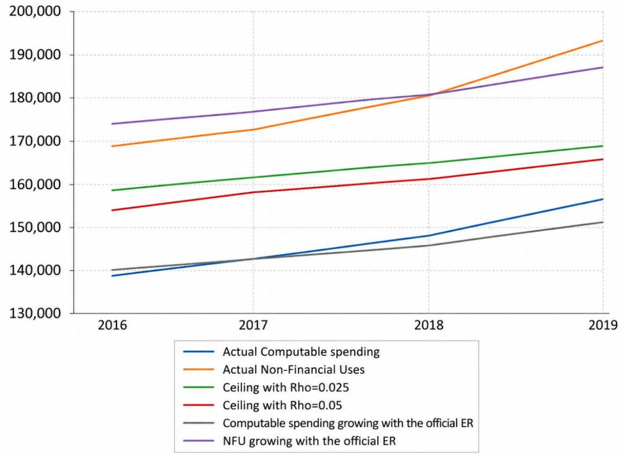
* Figures in millions of euros ** Source: authors and compliance reports.
Figure 5 exhibits a less stringent ceiling, even if still far from the NFU registered in the period, and again above the computable spending. In this regard, and according to differential factors of the fiscal position of ACs, this speed of adjustment could be also adapted at level of each AC, so that the debt convergence path becomes feasible and credible.
Modifying the long-term objective for public debt
Previous simulations have dealt with 13 percent of GDP as the level to be reached by all the ACs at the end of the debt reduction trajectory. However, this value, estimated at the time of the LOEPSF, might not necessarily be the most appropriate or realistic long-term reference for all the ACs. Determining the sustainable level of public debt for each AC’s would entail assuming certain assumptions for the fiscal policy stance, short/long term composition of debt, interest rates, etc. and, by simulating stochastic shocks, determine the “safe” level that could be the anchor of the fiscal rule (see Eyraud et al, 2018).
Such analysis is out of the scope of this paper but, for sake of comparison with the previous scenario, we present next how the ceiling would change if the target for regional public debt is set up at 20 percent of GDP for all ACs. In the case of those ACs that were below 20 percent at the beginning of the period, according to the expression (9), they will be allowed to enjoy an extra margin in their expenditure ceiling. Table 16 and Figure 7 report the results in the new scenario.
Similarly to the simulation with an enlarged debt consolidation period, the ceiling expenditure moves upwards. The regional governments would be allowed to spend more. Again, the circumstances of each AC could be considered in order to determine the long-term value towards they must move.
Table 16. Different expenditure ceilings depending on the long-term Debt/GDP target.
| Expenditure ceiling Debt*=13% GDP | Expenditure ceiling Debt*=20% GDP | |||||||
| 2016 | 2017 | 2018 | 2019 | 2016 | 2017 | 2018 | 2019 | |
| Andalucía | 24,782 | 25,979 | 27,175 | 28,368 | 25,289 | 26,461 | 27,632 | 28,803 |
| Aragón | 4,217 | 4,281 | 4,336 | 4,384 | 4,332 | 4,390 | 4,440 | 4,483 |
| Canarias | 7,499 | 7,548 | 7,589 | 7,624 | 7,641 | 7,683 | 7,717 | 7,746 |
| Cantabria | 2,182 | 2,198 | 2,211 | 2,221 | 2,225 | 2,239 | 2,250 | 2,258 |
| Castilla y León | 8,074 | 8,119 | 8,155 | 8,184 | 8,260 | 8,296 | 8,323 | 8,344 |
| Castilla-La Mancha | 5,681 | 5,795 | 5,895 | 5,983 | 5,811 | 5,919 | 6,012 | 6,094 |
| Cataluña | 24,638 | 25,933 | 27,223 | 28,507 | 25,354 | 26,613 | 27,869 | 29,120 |
| Comunidad de Madrid | 20,728 | 21,099 | 21,426 | 21,714 | 21,443 | 21,778 | 22,071 | 22,327 |
| Comunidad Foral de Navarra | 3,495 | 3,524 | 3,550 | 3,574 | 3,559 | 3,584 | 3,608 | 3,629 |
| Comunitat Valenciana | 13,692 | 14,456 | 15,217 | 15,974 | 14,042 | 14,789 | 15,533 | 16,275 |
| Extremadura | 4,052 | 4,074 | 4,092 | 4,107 | 4,114 | 4,134 | 4,149 | 4,161 |
| Galicia | 9,294 | 9,412 | 9,519 | 9,614 | 9,493 | 9,601 | 9,698 | 9,784 |
| Baleares | 4,401 | 4,725 | 5,048 | 5,371 | 4,500 | 4,819 | 5,138 | 5,456 |
| La Rioja | 1,151 | 1,166 | 1,178 | 1,188 | 1,179 | 1,192 | 1,203 | 1,212 |
| País Vasco | 9,674 | 9,985 | 10,296 | 10,606 | 9,902 | 10,201 | 10,501 | 10,801 |
| Principado de Asturias | 3,632 | 3,639 | 3,645 | 3,649 | 3,707 | 3,710 | 3,712 | 3,713 |
| Región de Murcia | 4,165 | 4,250 | 4,325 | 4,392 | 4,264 | 4,345 | 4,415 | 4,477 |
| total | 151,359 | 156,184 | 160,879 | 165,461 | 155,117 | 159,755 | 164,271 | 168,684 |
*In millions of Euros
**Source: authors
Figure 6: Different expenditure ceilings depending on the long-term debt target, NFUs, computable spending according to official ER, and actual computable spending
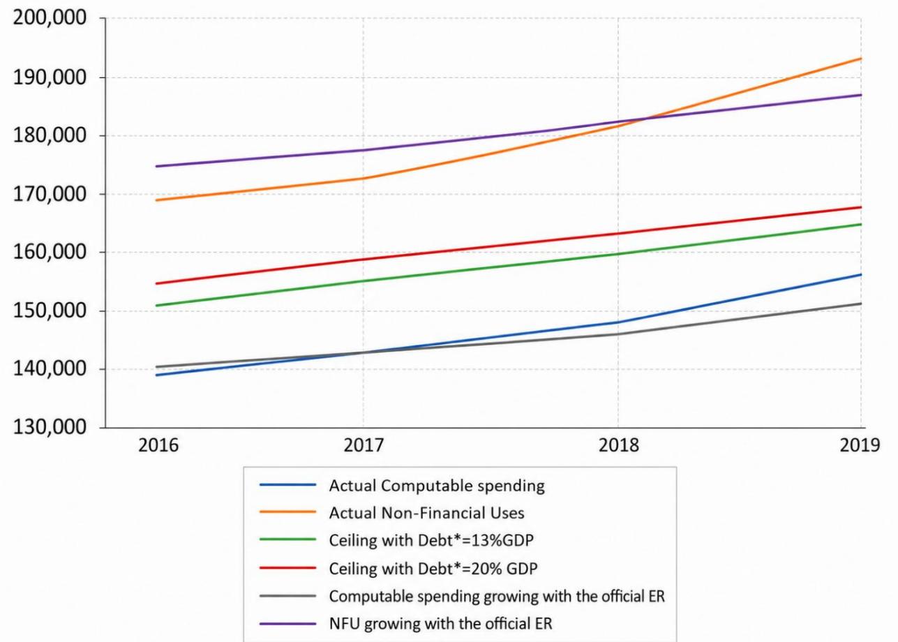
* In millions of euros ** Source: authors and compliance reports.
Establishing the rule over a different period.
A third way to address the problem of the stringency found in the first simulation is to start to apply the rule in a period when fiscal consolidation, at least in nominal terms, is completed. In fact, establishing transitional periods before the enforcement of new fiscal rules is a common practice in many jurisdictions, including in Spain, where the LOEPSF established a long transitional period. Implementing the new rule in a period with lower levels of deficits instead of the previously considered would be much less stringent, with differences between the ceiling derived from the rule and the actual expenditure being much lower.
We describe next a simulation for the period 2025-2028, starting at the level of regional public debt existing in December 2024. The policy parameters remain unchanged: speed of convergence ρ = 0.05 and the long-term debt target in 13 percent of the GDP. Table 17 informs also about the relevant levels of public debt and GDP.
Table 17. Initial debt level, period 2025-2028.
| $\rho=0.05$ | $D_{t0=2024}$ | $GDP_{t0=2024}$ | $D^{*}=13\%GDP_{t0=2024}$ | $Dt_0/GDP_{t0}$ | |
| Andalucía | 0.05 | 40,529 | 212,403 | 27,612 | 19% |
| Aragón | 0.05 | 9,402 | 49,580 | 6,445 | 19% |
| Canarias | 0.05 | 6,569 | 57,568 | 7,484 | 11% |
| Cantabria | 0.05 | 3,234 | 17,821 | 2,317 | 18% |
| Castilla y León | 0.05 | 14,239 | 75,290 | 9,788 | 19% |
| Castilla-La Mancha | 0.05 | 16,630 | 57,287 | 7,447 | 29% |
| Cataluña | 0.05 | 89,035 | 299,396 | 38,921 | 30% |
| Comunidad de Madrid | 0.05 | 37,260 | 311,319 | 40,471 | 12% |
| Comunidad Foral de Navarra | 0.05 | 2,745 | 26,601 | 3,458 | 10% |
| Comunitat Valenciana | 0.05 | 60,329 | 148,102 | 19,253 | 41% |
| Extremadura | 0.05 | 5,552 | 26,419 | 3,434 | 21% |
| Galicia | 0.05 | 11,936 | 82,173 | 10,683 | 15% |
| Baleares | 0.05 | 8,426 | 44,705 | 5,812 | 19% |
| La Rioja | 0.05 | 1,634 | 11,279 | 1,466 | 14% |
| País Vasco | 0.05 | 10,842 | 93,328 | 12,133 | 12% |
| Principado de Asturias | 0.05 | 4,066 | 30,089 | 3,912 | 14% |
| Región de Murcia | 0.05 | 13,513 | 42,901 | 5,577 | 31% |
| total | 0.05 | 335,944 | 1,586,262 | 206,214 | 21% |
*In millions of Euros **Source: Authors from Banco de España and INE
We again estimate the trend-revenue using the HW method, but in this case, we will assign a parameter which ranks in the middle of the two extreme cases presented before (α = 0.25 and α = 0.9), but still giving more weight to recent observations of the revenue series against the most remote past. Particularly, we are considering that α = 0.7. Table 18 shows the smoothing parameters estimated according to the AIC criterion for the total of ACs. Figure 8 illustrates the dynamics of actual and smoothed revenues, with a projection over the period 2025-2028.
Table 18: Estimates and AIC criterion for HW smoothing with α = 0.7. Total ACs, 2025-2028
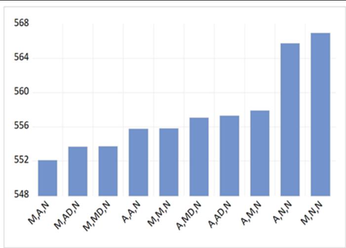
*Source: Authors
ETS Smoothing Original series: TOTAL Date: 02/06/26 Time: 09:57 Sample: 2000 2028 Included observations: 25 Model: M,A,N - Multiplicative Error, Additive Trend, No Season (Auto E=*, T=*) Model selection: Akaike Information Criterion Convergence achieved after 6 iterations
| Parameters | |
| Alpha (fixed): | 0.700000 |
| Beta: | 0.131110 |
| Initial Parameters | |
| Initial level: | 61496.17 |
| Initial trend: | 10647.91 |
| Compact Log-likelihood | -274.0604 |
| Log-likelihood | -269.2979 |
| Akaike Information Criterion | 552.1207 |
| Schwarz Criterion | 554.5585 |
| Hannan-Quinn Criterion | 552.7969 |
| Sum of Squared Residuals | 0.141482 |
| Root Mean Squared Error | 0.075228 |
| Average Mean Squared Error | 3.24E+08 |
Figure 7: Projection for period 2025-2028 and smoothing
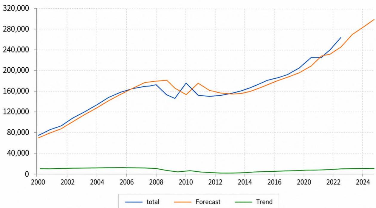
*In millions of euros **Source: Authors
On this basis and using again the expression (9), the Table 19 reports the estimated trend-revenue series and the corresponding expenditure ceilings for the whole of Spanish regional governments.
Table 19: Trend Revenue (α=0.7) and ceiling according to expression (9)
| TRt, Trend Revenue (a=07) | Expenditure ceiling according to proposal | |||||||
| 2025 | 2026 | 2027 | 2028 | 2025 | 2026 | 2027 | 2028 | |
| Andalucía | 40,258 | 41,467 | 42,676 | 43,885 | 39,612 | 40,853 | 42,093 | 43,331 |
| Aragón | 7,084 | 7,118 | 7,149 | 7,176 | 6,936 | 6,978 | 7,015 | 7,049 |
| Canarias | 14,409 | 15,241 | 16,072 | 16,903 | 14,455 | 15,284 | 16,113 | 16,943 |
| Cantabria | 3,601 | 3,731 | 3,833 | 3,914 | 3,555 | 3,687 | 3,792 | 3,875 |
| Castilla y León | 12,944 | 13,203 | 13,408 | 13,568 | 12,721 | 12,992 | 13,207 | 13,378 |
| Castilla-La Mancha | 9,634 | 9,797 | 9,924 | 10,022 | 9,175 | 9,361 | 9,509 | 9,628 |
| Cataluña | 48,155 | 49,527 | 50,898 | 52,270 | 45,649 | 47,146 | 48,637 | 50,122 |
| Comunidad de Madrid | 38,968 | 40,262 | 41,556 | 42,850 | 39,129 | 40,414 | 41,701 | 42,987 |
| Comunidad Foral de Navarra | 6,590 | 6,823 | 6,991 | 7,112 | 6,626 | 6,857 | 7,023 | 7,142 |
| Comunitat Valenciana | 25,681 | 26,438 | 27,194 | 27,950 | 23,628 | 24,486 | 25,340 | 26,189 |
| Extremadura | 6,597 | 6,897 | 7,151 | 7,368 | 6,491 | 6,796 | 7,056 | 7,277 |
| Galicia | 14,516 | 14,882 | 15,248 | 15,614 | 14,453 | 14,822 | 15,191 | 15,560 |
| Baleares | 8,037 | 8,347 | 8,657 | 8,967 | 7,906 | 8,223 | 8,539 | 8,855 |
| La Rioja | 2,045 | 2,159 | 2,272 | 2,386 | 2,037 | 2,151 | 2,265 | 2,379 |
| País Vasco | 14,726 | 15,090 | 15,455 | 15,820 | 14,790 | 15,152 | 15,514 | 15,876 |
| Principado de Asturias | 5,852 | 5,981 | 6,070 | 6,132 | 5,845 | 5,973 | 6,063 | 6,125 |
| Región de Murcia | 7,126 | 7,181 | 7,232 | 7,278 | 6,729 | 6,804 | 6,874 | 6,938 |
| total | 266,224 | 274,143 | 281,786 | 289,214 | 259,738 | 267,981 | 275,932 | 283,652 |
*In millions of Euros **Source: Authors
Table 20. Comparison growth rates in ceiling and official proposed reference rates, in percentage
| Expenditure Growth according to proposal | Official rates proposed by Government | |||||
| 2026 | 2026 | 2028 | 2026 | 2027 | 2028 | |
| Andalucía | 3.1 | 3.0 | 2.9 | 3.5 | 3.4 | 3.2 |
| Aragón | 0.6 | 0.5 | 0.5 | 3.5 | 3.4 | 3.2 |
| Canarias | 5.7 | 5.4 | 5.1 | 3.5 | 3.4 | 3.2 |
| Cantabria | 3.7 | 2.8 | 2.2 | 3.5 | 3.4 | 3.2 |
| Castilla y León | 2.1 | 1.7 | 1.3 | 3.5 | 3.4 | 3.2 |
| Castilla-La Mancha | 2.0 | 1.6 | 1.2 | 3.5 | 3.4 | 3.2 |
| Cataluña | 3.3 | 3.2 | 3.1 | 3.5 | 3.4 | 3.2 |
| Comunidad de Madrid | 3.3 | 3.2 | 3.1 | 3.5 | 3.4 | 3.2 |
| Comunidad Foral de Navarra | 3.5 | 2.4 | 1.7 | 3.5 | 3.4 | 3.2 |
| Comunitat Valenciana | 3.6 | 3.5 | 3.3 | 3.5 | 3.4 | 3.2 |
| Extremadura | 4.7 | 3.8 | 3.1 | 3.5 | 3.4 | 3.2 |
| Galicia | 2.6 | 2.5 | 2.4 | 3.5 | 3.4 | 3.2 |
| Baleares | 4.0 | 3.8 | 3.7 | 3.5 | 3.4 | 3.2 |
| La Rioja | 5.6 | 5.3 | 5.0 | 3.5 | 3.4 | 3.2 |
| País Vasco | 2.4 | 2.4 | 2.3 | 3.5 | 3.4 | 3.2 |
| Principado de Asturias | 2.2 | 1.5 | 1.0 | 3.5 | 3.4 | 3.2 |
| Región de Murcia | 1.1 | 1.0 | 0.9 | 3.5 | 3.4 | 3.2 |
| total | 3.2 | 3.0 | 2.8 | 3.5 | 3.4 | 3.2 |
Source: Authors
Table 20 compares the growth rates derived from the expenditure ceilings of Table 19 with the reference rates proposed by the government for years 2026-202810. Focusing on the aggregate figure, the growth rates are not very different, slightly tighter the proposal than the officially proposed reference rates. At the individual level, differences across the ACs arise, depending upon the past trend of revenues and initial level of debt in 2024 by comparison to the 13 percent of GDP.
We also provide a comparison between the budget balance that would be achieved if the revenues were to coincide exactly with the estimated trend revenues and the expenditure coinciding with the ceiling. Under such case, the budgetary surplus would be just the right part of the expression (9), i.e., the resources devoted to reducing debt. These estimates are compared to the targets proposed by the Government in Table 21.
10 Agreement of the Government (Council of Ministers), November 18th, 2025. https://www.congreso.es/backoffice_doc/atp/odiapleno_textos/430.8.pdf
Table 21. Comparison budget balance if strict compliance with the rule and actual revenues equaling trendrevenues, against the officially proposed budget targets, in percentage
| fiscal balance if strict compliance with the ceiling | Officially proposed deficit targets | |||||||
| 2025 | 2026 | 2027 | 2028 | 2025 | 2026 | 2027 | 2028 | |
| Andalucía | 0.3 | 0.3 | 0.2 | 0.2 | 0.1 | -0.1 | -0.1 | -0.1 |
| Aragón | 0.3 | 0.3 | 0.2 | 0.2 | 0.1 | -0.1 | -0.1 | -0.1 |
| Canarias | -0.1 | -0.1 | -0.1 | -0.1 | 0.1 | -0.1 | -0.1 | -0.1 |
| Cantabria | 0.2 | 0.2 | 0.2 | 0.2 | 0.1 | -0.1 | -0.1 | -0.1 |
| Castilla y León | 0.3 | 0.3 | 0.2 | 0.2 | 0.1 | -0.1 | -0.1 | -0.1 |
| Castilla-La Mancha | 0.8 | 0.7 | 0.6 | 0.6 | 0.1 | -0.1 | -0.1 | -0.1 |
| Cataluña | 0.8 | 0.7 | 0.7 | 0.6 | 0.1 | -0.1 | -0.1 | -0.1 |
| Comunidad de Madrid | 0.0 | 0.0 | 0.0 | 0.0 | 0.1 | -0.1 | -0.1 | -0.1 |
| Comunidad Foral de Navarra | -0.1 | -0.1 | -0.1 | -0.1 | 0.1 | -0.1 | -0.1 | -0.1 |
| Comunitat Valenciana | 1.3 | 1.2 | 1.1 | 1.0 | 0.1 | -0.1 | -0.1 | -0.1 |
| Extremadura | 0.4 | 0.3 | 0.3 | 0.3 | 0.1 | -0.1 | -0.1 | -0.1 |
| Galicia | 0.1 | 0.1 | 0.1 | 0.1 | 0.1 | -0.1 | -0.1 | -0.1 |
| Baleares | 0.3 | 0.3 | 0.2 | 0.2 | 0.1 | -0.1 | -0.1 | -0.1 |
| La Rioja | 0.1 | 0.1 | 0.1 | 0.1 | 0.1 | -0.1 | -0.1 | -0.1 |
| País Vasco | -0.1 | -0.1 | -0.1 | -0.1 | 0.1 | -0.1 | -0.1 | -0.1 |
| Principado de Asturias | 0.0 | 0.0 | 0.0 | 0.0 | 0.1 | -0.1 | -0.1 | -0.1 |
| Región de Murcia | 0.9 | 0.8 | 0.7 | 0.7 | 0.1 | -0.1 | -0.1 | -0.1 |
| total | 0.4 | 0.4 | 0.3 | 0.3 | 0.1 | -0.1 | -0.1 | -0.1 |
*Source: Authors
Although at aggregate level the proposed rule would be slightly more stringent than the currently existing one, the individual targets do not differ too much from those proposed by the Government. The main differences appear in those ACs with a higher stock of public debt and more need to reach a higher surplus. But in general, as assumed, if the rule is to be established in a moment when ACs budgets are virtually in balance, no stringent features are found at all, if compared to the set up by the government.
In terms of public debt reduction, the new rule would achieve the same result obtained in the simulation carried out over the period 2016-2019, as the Table 22 shows. Recalling that there was a reduction in the public-to-GDP ratio by almost 5 percentual points on average; that involves around one fifth of the initial stock of debt as share of GDP.
Table 22. Debt reduction according to proposal, in percentage
| 2024(Actual) | 2025 | 2026 | 2027 | 2028 | total | in percentage of initial debt/GDP | |
| Andalucía | 19.1 | 17.8 | 16.8 | 15.9 | 15.2 | -3.9 | -20.6 |
| Aragón | 19.0 | 17.7 | 16.7 | 15.8 | 15.1 | -3.9 | -20.5 |
| Canarias | 11.4 | 10.9 | 10.5 | 10.2 | 9.9 | -1.5 | -13.4 |
| Cantabria | 18.1 | 17.0 | 16.1 | 15.2 | 14.5 | -3.6 | -20.0 |
| Castilla y León | 18.9 | 17.7 | 16.7 | 15.8 | 15.0 | -3.9 | -20.5 |
| Castilla-La Mancha | 29.0 | 26.8 | 25.0 | 23.4 | 22.0 | -7.0 | -24.2 |
| Cataluña | 29.7 | 27.4 | 25.6 | 23.9 | 22.5 | -7.3 | -24.4 |
| Comunidad de Madrid | 12.0 | 11.4 | 11.0 | 10.6 | 10.3 | -1.7 | -14.2 |
| Comunidad Foral de Navarra | 10.3 | 9.9 | 9.6 | 9.4 | 9.1 | -1.2 | -11.5 |
| Comunitat Valenciana | 40.7 | 37.4 | 34.6 | 32.2 | 30.0 | -10.7 | -26.2 |
| Extremadura | 21.0 | 19.6 | 18.4 | 17.4 | 16.5 | -4.5 | -21.5 |
| Galicia | 14.5 | 13.7 | 13.1 | 12.5 | 12.0 | -2.5 | -17.2 |
| Baleares | 18.8 | 17.6 | 16.6 | 15.8 | 15.0 | -3.9 | -20.4 |
| La Rioja | 14.5 | 13.7 | 13.1 | 12.5 | 12.0 | -2.5 | -17.2 |
| País Vasco | 11.6 | 11.1 | 10.7 | 10.3 | 10.0 | -1.6 | -13.7 |
| Principado de Asturias | 13.5 | 12.8 | 12.3 | 11.8 | 11.3 | -2.2 | -16.2 |
| Región de Murcia | 31.5 | 29.0 | 27.0 | 25.2 | 23.7 | -7.8 | -24.8 |
| total | 21.2 | 19.7 | 18.6 | 17.5 | 16.6 | -4.6 | -21.6 |
*In percetage of the GDP and percentual change **Source: Authors, Banco de España, with GDP estimated figures from the Medium-Term Fiscal Structural Plan
Using different smoothing-projection parameters
We have found that, obviously, the estimated trend revenue and, consequently the expenditure ceilings are not neutral to the methodology for smoothing and forecasting used. Particularly, depending on the value for the parameter α when smoothing revenues, the projection may have lower or higher slope, and therefore, regional governments are allowed to spend more or less. But more importantly, this apparently discretional autonomy to decide ultimately the expenditure ceilings can be redirected to introduce incentives to increase the own resources of the ACs. The new European fiscal rules precisely try to do the same when allow for higher expenditure in the case of permanent or transitory increases of tax collection.
To illustrate this issue, we refer to a recent study by the Banco de Espana (2025). This paper starts from the current situation, in which the resources from inheritance and gift taxes accounted for 0.23 percent of GDP in 2023. On this basis, the authors assume that all the Spanish regions set to set their tax parameters at the levels established by the national benchmark law. As result of this, revenues could increase by 0.5 percentage points of GDP, reaching 0.7% of GDP.
This quantification is based on the assumption that the modifications introduced to the tax would not induce substantial changes in the behavior of economic agents. In numerical terms, this means that if they were to introduce this change in 2023, ACs non-financial revenues could increase in 2024, by around 7,669 million euros. In the following Figure 9 we compare how the smoothed revenue series provided by the HW filter are affected in the next four scenarios, which are parallel to the scenarios presented in the two main simulations, but considering the change in the inheritance and gift tax:
1. No change in inheritance and gift tax, and ;
2. No change in inheritance and gift tax and and
3. Change in inheritance and gift tax, yielding an increase in the total revenues for ACs of 7,669 million euros in 2024 and ;
4. Change in inheritance and gift tax, producing an increase in the total for ACs of 7,669 million euros in 2024 and and
Figure 8: Different trend-revenues depending on and tax collection
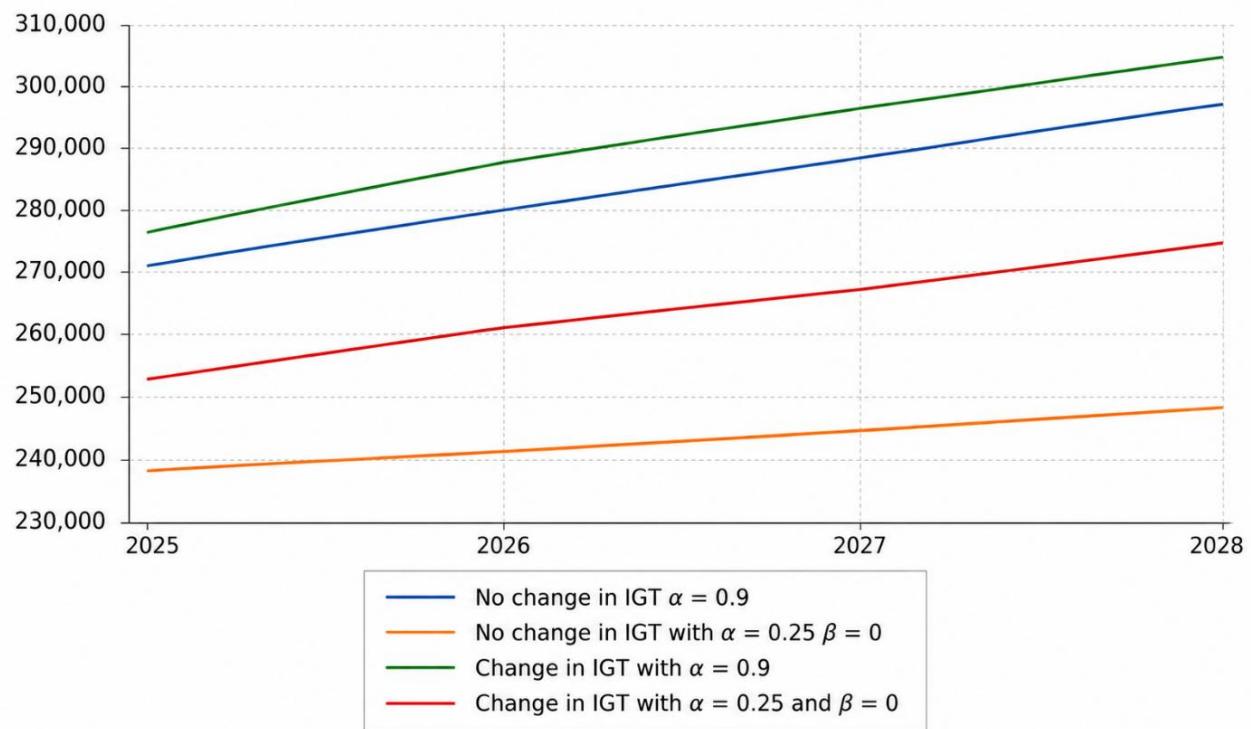
*In millions of euros **Source: Authors
The increase in tax collection allows for a higher ceiling in the case of a higher value of α. If we were to consider simultaneously the sensitivity of the ceiling to the parameter corresponding to the trend and to the level and give a relatively high value to both parameters, the ceiling would be even higher. In figure 9 we see that with both parameters at 0.7, the ceiling is substantially higher in the case of the change in tax collection and even higher (around 5% on average) than in the case of
Figure 9: Different trend-revenues with high levels of both parameters α and and different levels of tax collection.
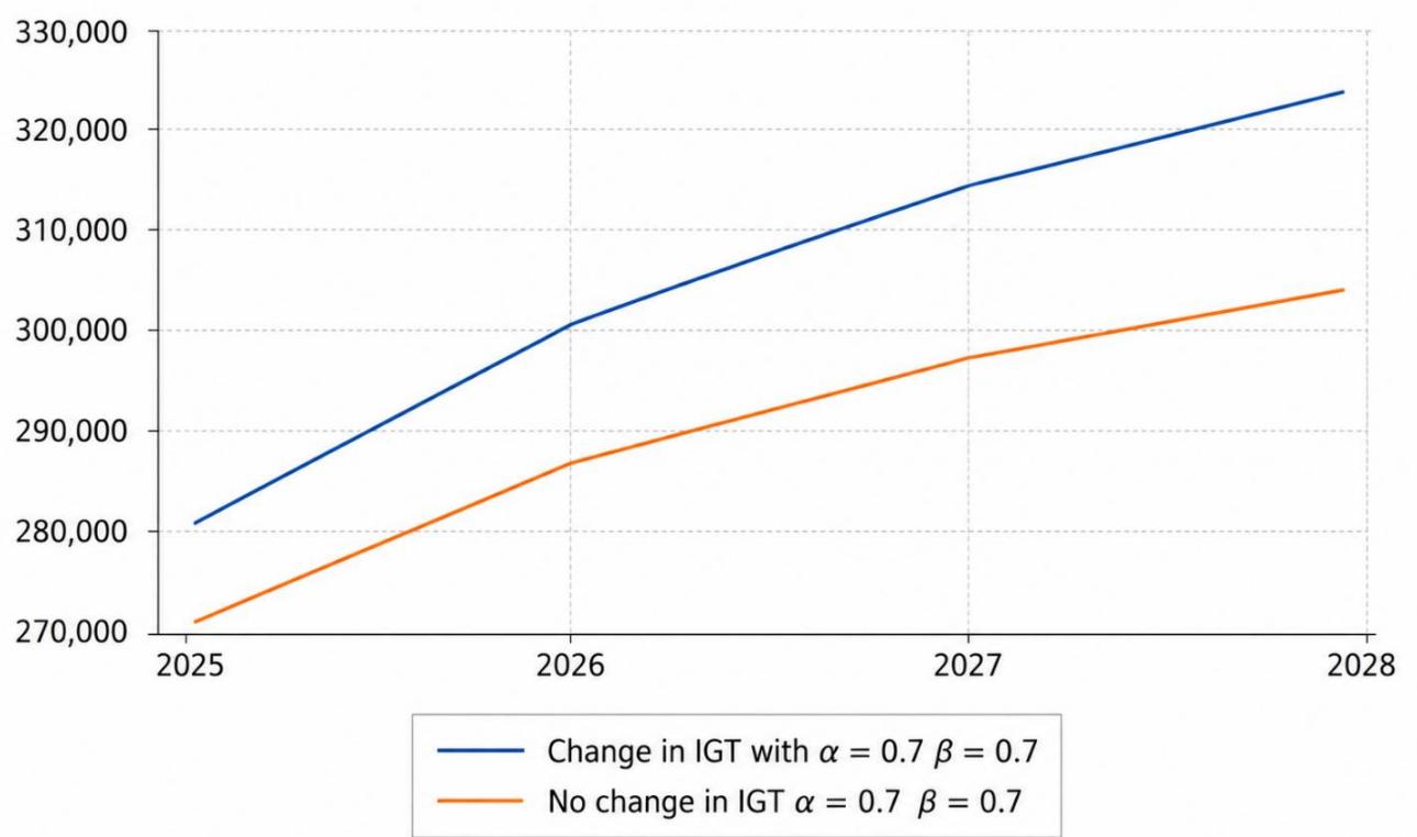
*In millions of euros **Source: Authors
By using a high value for the parameters α and increases in tax collection translate into higher ceilings, thereby creating incentives from the revenue side. And the higher the value of the parameters, the higher the ceiling and therefore, the higher the incentives to increase own revenues.
We have deliberately not suggested any best value for the and parameters or the long-term debt target. We are of the view that these values need to be determined in view of the specific circumstances of each AC, in line with the new EU fiscal governance, that tailor adjustments to the specific circumstances of each country. For example, there seems to be a consensus that the Autonomous financing system has played a role in certain vertical or horizontal imbalances, that may have had an impact on the fiscal performance of ACs and their current stock of debt. We cannot therefore suggest any best values for all the ACs. But the proposed rule is flexible enough to take into consideration these factors by, for instance, considering different debt consolidation paths or the power to increase the own resources and whether the AC has used its tax autonomy in previous years.
In this sense, we are of the view that the play of an independent authority (AIReF) would be a fundamental piece in a new governance based upon this new fiscal rule, since it has the technical capacity to determine long-term debt targets for each AC and to determine the rest of the parameters according to the economic reality of each AC. It would also avoid political economy problems observed when the Central Government proposed fiscal objectives to the ACs. These political economy problems might explain, for example, the fact that since a decade ago, the central government proposes systematically a common deficit objective (not an individual one). Giving this responsibility to AIReF would reduce this political pressure at the central government and its role would be more of a coordinator of the regional level with the general government fiscal framework.
Other refinements of the rule could address other problems of the current fiscal rules. For example, we have explained how the play of the smoothing parameter α can induce incentives to exploit ACs tax autonomy. But increases in the ceiling could also be granted if there are structural reforms that are going to create important long-term gains as it happens in the EU framework or to reflect increases in the investment expenditure, an aspect that needs further improvement in the current framework, where the “financially sustainable investments” have not been able to protect capital expenditure in economic downturns.
8. Concluding remarks
We have proposed a fiscal rule that departs from a very simple idea: the expenditure should follow the long-term trend of the revenue, corrected by a predetermined trajectory of debt reduction. The first advantage of the proposed rule is that we would gain in simplicity: one single rule could substitute the current set of three rules in the Spanish framework of fiscal governance. Another important difference between this proposal and the current set of rules is that compliance is assessed over a multi-year period, therefore avoiding the possibility of consolidating expenditure in non-compliance episodes. The rule allows for adjustments over a multi-year period, making it more credible and easier to monitor and enforce.
Considering the relatively high volatility of revenue of Spanish regional governments, this rule in principle would likely entail that the budget balance could be more volatile than it is with the current fiscal rules. However, we have linked the level of expenditure to a smoothed trajectory of revenues, previously estimated using the Holt-Winters filter. This way, regional public expenditures would remain more stable and growing or decreasing in a smooth fashion. This stability of expenditure is also an interesting property for budgetary planning.
The proposal also makes the rule more fit to the individual fiscal situation of each AC, since it establishes an individual spending ceiling based on their past revenue trends and the necessary debt reduction to achieve the target debt level. The use of revenue-based ceilings rather than GDP also strengthens the link between public spending and the fiscal autonomy of each AC, creating incentives to increase revenues when the regional governments decide to spend more.
It also contains some countercyclical properties, so that when revenues exceed the smoothed trend, surpluses are generated because public expenditures are subject to a ceiling, and vice versa. And this will happen despite the fact of being aimed at reaching fiscal balances in the medium/long term. Additional provisions regarding the use of surpluses to further reductions in public debt are worth considering.
One could argue that, as the simulation showed and for sake of stringency, the proposed rule can be difficult to establish in certain circumstances of fiscal consolidation. However, this issue can be addressed by modifying accordingly the debt reduction path, the long-term debt objective or starting to apply the rule in a time when AC are in fiscal balance, after a transitional period.
In any event, and this is the most important feature of the proposed rule, it allows for a predictable reduction in the stock of regional public debt, in contrast with the current set of rules, which has not contributed to debt reduction at the AC level. The proposed rule would allow for sufficient fiscal space to bring the stock of debt to the desired level in a determined number of years. The speed of adjustment or the target for the level of debt are matters for technical analyses and political decisions that go beyond the scope of this paper.
Further research related to this proposal could include the management of possible noncompliance with the rule after the expiration of the period corresponding to the ceiling or whether the total non-financial resources are the most adequate variable for measuring compliance with the rule. In this sense, certain studies (Ardanaz et al. 2020), point to the fact that rules that exclude investment expenditure tend to protect better this expenditure over the cycle.
References
- Alonso, V., Arroyo, C., Aydin, O., Balasundharam, V., Davoodi, H. R., Hegab, G., Nguyen, A. M., Salazar Ferro, N., Sher, G., Solovyeva, A., & Tchelishvili, N. (2025). Fiscal rules and fiscal councils: Recent trends and revisions since the pandemic (IMF Working Paper No. 25/198). International Monetary Fund, Washington, DC.
- Andrle, M., Bluedorn, J., Eyraud, L., Kinda, T., Koeva Brooks, P., Schwartz, G., & Weber, A. (2015). Reforming fiscal governance in the European Union (IMF Staff Discussion Note No. 15/09). International Monetary Fund, Washington, DC.
- Ardanaz, M., Cavallo, E., Izquierdo, A., & Puig, J. (2020). Growth-friendly fiscal rules? Safeguarding public investment from budget cuts through fiscal rule design (Fiscal Management Division). Inter-American Development Bank.
- Autoridad Independiente de Responsabilidad Fiscal. (2015). La regla de gasto y la sostenibilidad de las finanzas públicas (Documento divulgativo, 20 de noviembre de 2015).
- Autoridad Independiente de Responsabilidad Fiscal. (2016). Informe sobre el establecimiento de los objetivos individuales de estabilidad presupuestaria y deuda pública para las comunidades autónomas.
- Autoridad Independiente de Responsabilidad Fiscal. (2019). Observatorio de deuda (noviembre 2019).
- Autoridad Independiente de Responsabilidad Fiscal. (2022). Reforma del marco de gobernanza fiscal: una propuesta para España de ancla de deuda y regla de gasto. Documento Técnico 3/22
- Autoridad Independiente de Responsabilidad Fiscal. (2023). Observatorio de deuda (abril 2023).
- Autoridad Independiente de Responsabilidad Fiscal. (2024). Informe sobre el plan fiscal y estructural de medio plazo 2025–2028 (Informe 51/24, 5 de noviembre de 2024).
- Autoridad Independiente de Responsabilidad Fiscal. (2025). Opinión sobre la reforma del marco fiscal nacional (Opinión 4/25, 24 de noviembre de 2025).
- Badinger, H., & Reuter, W. (2017). The case for fiscal rules. Economic Modelling, 60, 334–343.
- Banco Central Europeo. (2016). Government debt reduction strategies in the euro area (ECB Economic Bulletin, Issue 3).
- Barkema, J., Gudmundsson, T., & Mrkaic, M. (2020). What do we talk about when we talk about output gaps? (IMF Working Paper No. 20/259). International Monetary Fund.
- Baskaran, T. (2012). Soft budget constraints and strategic interactions in subnational borrowing: Evidence from the German states, 1975–2005. Journal of Urban Economics, 71(1), 114–127.
- Brändle, T., & Elsener, M. (2024). Do fiscal rules matter? A survey of recent evidence. Swiss Journal of Economics and Statistics, 160(11).
- Calvo, S., & Cadaval, M. (2022). The impact of soft budget constraint on the fiscal coresponsibility of the autonomous communities in Spain: The case of extraordinary liquidity funds (2012–2019). Hacienda Pública Española/Review of Public Economics, 240(1), 151–190.
- Christofzik, D., Feld, L. P., Reuter, W. H., & Yeter, M. (2018). Uniting European fiscal rules: How to strengthen the fiscal framework (ZBW Working Paper No. 04/2018).
- Comisión Europea. (2019). Vade mecum on the stability and growth pact (Institutional Paper 101).
- Comisión Europea. (2020). Economic governance review. https://economyfinance.ec.europa.eu/economic-and-fiscal-governance/economic-governance-review_en
- Cordes, T., Kinda, T., Muthoora, P., & Weber, A. (2015). Expenditure rules: Effective tools for sound fiscal policy? (IMF Working Paper No. 15/29). International Monetary Fund.
- Cuenca, A. (2015). Las comunidades autónomas en 2015: Estabilidad presupuestaria y sostenibilidad financiera. Cuadernos de Información Económica, 246, 47–58.
- Căpraru, B., Pappas, A., & Sprincean, N. (2024). Fiscal rules in the European Union: Less is more. Journal of Common Market Studies, 63, 320-334.
- Davoodi, H. R., Eladari, P., Fotiou, A., Garcia-Macia, D., Lagerborg, A., Raphael, L., & Pillai, S. (2022). Fiscal rules dataset: 1985–2021 (IMF Working Paper No. 2022/011). International Monetary Fund.
- Debrun, X., Epstein, N., & Symansky, S. (2008). A new fiscal rule: Should Israel go Swiss? (IMF Working Paper No. 2008/87). International Monetary Fund.
- Delgado-Téllez, M., Gordo, E., Kataryniuk, I., & Pérez, J. J. (2020). The decline in public investment: Social dominance or too-rigid fiscal rules? (Banco de España Working Paper No. 2025). Banco de España.
- European Fiscal Board. (2019). Assessment of EU fiscal rules with a focus on the six- and twopack legislation (August 2019).
- Eyraud, L., Debrun, M. X., Hodge, A., Lledó, V. D., & Pattillo, C. A. (2018). Second-generation fiscal rules: Balancing simplicity, flexibility, and enforceability. (IMF Working Paper No. 2018/4) International Monetary Fund.
- Eyraud, L., Hodge, A., Ralyea, J., & Reynaud, J. (2020). How to design subnational fiscal rules: A primer. (IMF Note 2020/1) International Monetary Fund.
- Fernández-Huertas, I., Carrasco, R. y A. Díaz (2026). «El cumplimiento de la regla de gasto en las comunidades autónomas». Working Papers Ivie n.º 2026-1. València: Ivie.
- Fernández-Leiceaga, X., & Lago-Peñas, S. (2013). Sobre el reparto de los derechos de déficit entre comunidades autónomas: Una propuesta alternativa. Revista de Economía Aplicada, 63, 117–136.
- Fernández-Llera, R. (2016). Control del endeudamiento autonómico y estabilidad presupuestaria: Evolución y propuestas de futuro. Revista de Estudios Regionales, 105, 103–136.
- Fernández-Llera, R., & Monasterio, C. (2010). ¿Entre dos o entre todos? Examen y propuestas para la coordinación presupuestaria en España. Hacienda Pública Española/Review of Public Economics, 195(4), 139–163.
- Gadea, M. D., Gómez-Loscos, A., & Montañés, A. (2012). Cycles inside cycles: Spanish regional aggregation. SERIEs, 3(4), 423–456.
- Gardner, E. S. (2006). Exponential smoothing: The state of the art—Part II. International Journal of Forecasting, 22(4), 637–666.
- Gardner, E. S., & McKenzie, E. (2011). Why the damped trend works. Journal of the Operational Research Society, 62(6), 1177-1180.
- Ghosh, A. R., Kim, J. I., Mendoza, E. G., Ostry, J. D., & Qureshi, M. S. (2013). Fiscal fatigue, fiscal space and debt sustainability in advanced economies. The Economic Journal, 123(566), F4– F30.
- González, F., & Martínez-López, D. (2021). El diseño de reglas fiscales en gobiernos subcentrales: El caso de España. Fedea Policy Paper 2021/01.
- Goodspeed, T. J. (2017). Bailouts and soft budget constraints in decentralized government. Hacienda Pública Española/Review of Public Economics, 221(2), 113–134.
- Hauptmeier, S., & Kamps, C. (2020). Debt rule design in theory and practice: The SGP’s debt benchmark revisited (ECB Working Paper No. 2379).
- Heinemann, F., Moessinger, M. D., & Yeter, M. (2018). Do fiscal rules constrain fiscal policy? A meta-regression analysis. European Journal of Political Economy, 51, 69–92.
- House, C. L., Proebsting, C., & Tesar, L. L. (2020). Austerity in the aftermath of the Great Recession. Journal of Monetary Economics, 115, 37-63.
- Hyndman, R. J., Koehler, A. B., Ord, J. K. & Snyder, R. D. (2008). Forecasting with exponential smoothing: The state space approach. Springer: Berlin.
- Instituto Valenciano de Investigaciones Económicas. (2018). Deuda pública de las comunidades autónomas (Papeles de Financiación Autonómica No. 4/2018).
- Lago, S., Leiceaga, X., & Vaquero, A. (2017). ¿Por qué incumplen fiscalmente las comunidades autónomas? Investigaciones Regionales/Journal of Regional Research, 37, 7–29.
- Lago, S., Vaquero, A., Sánchez, P., & López, B. (2019). Does fiscal consolidation hurt economic growth? Empirical evidence from Spanish regions. Economics: The Open-Access, Open-Assessment E-Journal, 13, 1–19.
- Makridakis, S., & Hibon, M. (2000). The M3-competition: Results, conclusions and implications. International Journal of Forecasting, 16(4), 451–476.
- Makridakis, S., Spiliotis, E., & Assimakopoulos, V. (2020). The M4 competition: 100,000 time series and 61 forecasting methods. International Journal of Forecasting, 36(1), 54–74.
- Martínez-López, D. (2020). La gobernanza fiscal de las comunidades autónomas. Investigaciones Regionales/Journal of Regional Research, 47, 31–56.
- Martínez-López, D. (2022). Subnational borrowing and bailouts: When the federal government looks at the votes (differently) and its borrowing matters. Journal of Public Economic Theory, 24(3), 609–633.
- Martínez-López, D. & González, F. (2022). Los objetivos de déficit en las Comunidades Autónomas: una propuesta basada en la deuda. Hacienda Pública Española/Review of Public Economics, 241, 105-141.
- Martínez-López, D., González, F., & Porrero Ramírez, P. (2026). Propuesta para adaptar el marco español a la nueva gobernanza de la Unión Europea. FEDEA Estudios de Economía Española No. 2026-04.
- Marín, C. (2020). Descomposición de los saldos presupuestarios de las CCAA 2014–2018. FEDEA Estudios de Economía Española No. 2020-02.
- Marín-González, C., & Martínez-López, D. (2025). Fiscal stabilization, debt sustainability, and public spending in subnational governments: The case of the Spanish regions. Regional & Federal Studies, 36(2), 1–35.
- Medas, P., & González, C. (2023). The current reform process of fiscal rules: Lessons from an international perspective. Papeles de Economía Española, 175, 42-55.
- Melián, A., Quesada, M. L., & Velayos, J. (2015). La fijación de los objetivos de estabilidad presupuestaria y el déficit estructural. Crónica Presupuestaria, 3, 112–129.
- Micó, A., & Ramos, R. (2025). El posible impacto recaudatorio de algunas reformas hipotéticas del impuesto sobre sucesiones y donaciones. Banco de España, Boletín Económico 2025/T3.
- Ministerio de Hacienda. (varios años). Informe sobre el grado de cumplimiento de los objetivos de estabilidad presupuestaria y de deuda pública y de la regla de gasto.
- Ministerio de Hacienda. (varios años). Liquidación de los recursos del sistema de financiación de las comunidades autónomas de régimen común y ciudades con estatuto de autonomía.
- OECD. (2020). The territorial impact of COVID-19: Managing the crisis across levels of government. OECD Publishing.
- Salvi, M., Schaltegger, C., & Schmid, L. (2020). Fiscal rules cause lower debt: Evidence from Switzerland’s federal debt containment rule. Kyklos, 73(4), 605–642.
- Tax Policy Center. (2024). What are state rainy-day funds and how do they work? https://taxpolicycenter.org/briefing-book/what-are-state-rainy-day-funds-and-how-do-they-work
- Zabalza, A., & López-Laborda, J. (2017). The uneasy coexistence of the Spanish foral and common regional finance systems. Investigaciones Regionales/Journal of Regional Research, 37, 119–152.
I: Debt reduction path, calcu
| $\rho=0.05$ | $D_{t0}=2015$ | $GDP_{t0}=2015$ | $D^{*}=13\%^{*}GDP_{t0}$ | $D_{t=0}/GDP_{t=0}$ | $Dt_0-D^*$ | $\alpha(Dt_0-D^*)$ | $\alpha(D_{t0}-(\alpha(D_{t0}.D^*))-D^*))$ | $\alpha(D_{t0}-(D_{t0}-(\alpha(D_{t0}-D^*))-D^*))-D^*)$ | $\alpha(D_{t0}-\alpha(D_{t0}-\alpha(D_{t0}-(\alpha(D_{t0}-D^*))-D^*))-D^*))-D^*))$ | |
| Andalucía | 0.05 | 31,643 | 144,859 | 18,832 | 21.8% | 12,811 | 641 | 609 | 578 | 549 |
| Aragón | 0.05 | 6,930 | 32,897 | 4,277 | 21.1% | 2,653 | 133 | 126 | 120 | 114 |
| Canarias | 0.05 | 6,663 | 40,596 | 5,277 | 16.4% | 1,386 | 69 | 66 | 63 | 59 |
| Cantabria | 0.05 | 2,677 | 12,336 | 1,604 | 21.7% | 1,074 | 54 | 51 | 48 | 46 |
| Castilla y León | 0.05 | 10,557 | 53,273 | 6,925 | 19.8% | 3,632 | 182 | 173 | 164 | 156 |
| Castilla-La Mancha | 0.05 | 13,426 | 37,138 | 4,828 | 36.2% | 8,598 | 430 | 408 | 388 | 369 |
| Cataluña | 0.05 | 72,675 | 204,481 | 26,583 | 35.5% | 46,092 | 2,305 | 2,189 | 2,080 | 1,976 |
| Comunidad de Madrid | 0.05 | 28,683 | 204,158 | 26,540 | 14.0% | 2,143 | 107 | 102 | 97 | 92 |
| Comunidad Foral de Navarra | 0.05 | 3,322 | 18,154 | 2,360 | 18.3% | 962 | 48 | 46 | 43 | 41 |
| Comunitat Valenciana | 0.05 | 42,003 | 100,186 | 13,024 | 41.9% | 28,979 | 1,449 | 1,376 | 1,308 | 1,242 |
| Extremadura | 0.05 | 3,576 | 17,916 | 2,329 | 20.0% | 1,247 | 62 | 59 | 56 | 53 |
| Galicia | 0.05 | 10,375 | 56,698 | 7,371 | 18.3% | 3,004 | 150 | 143 | 136 | 129 |
| Baleares | 0.05 | 8,330 | 28,271 | 3,675 | 29.5% | 4,655 | 233 | 221 | 210 | 200 |
| La Rioja | 0.05 | 1,436 | 7,967 | 1,036 | 18.0% | 400 | 20 | 19 | 18 | 17 |
| País Vasco | 0.05 | 9,486 | 65,027 | 8,454 | 14.6% | 1,032 | 52 | 49 | 47 | 44 |
| Principado de Asturias | 0.05 | 3,876 | 21,389 | 2,781 | 18.1% | 1,096 | 55 | 52 | 49 | 47 |
| Región de Murcia | 0.05 | 7,601 | 28,509 | 3,706 | 26.7% | 3,895 | 195 | 185 | 176 | 167 |
| total | 0.05 | 263,259 | 1,073,854 | 139,601 | 24.5% | 123,658 | 6,183 | 5,874 | 5,580 | 5,301 |
Annex II: Holt-Winters smoothing and projection of revenues, statistics and AIC criterion, for each AC, α = 0.9
1. Andalucía
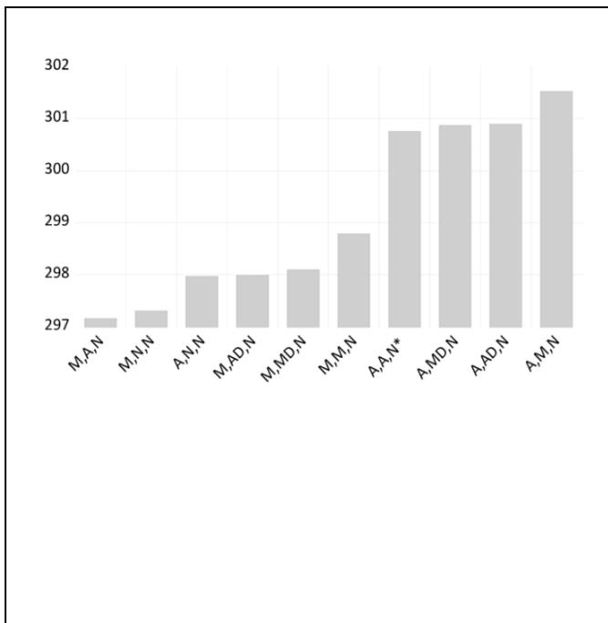
ETS Smoothing Original series: ANDALUCIA Date: 10/13/25 Time: 16:00 Sample: 2000 2019 Included observations: 16 Model: M,A,N - Multiplicative Error, Additive Trend, No Season (Auto E=*, T=*) Model selection: Akaike Information Criterion Convergence achieved after 1 iteration
| Parameters | |
| Alpha (fixed): | 0.900000 |
| Beta: | 0.000000 |
| Initial Parameters | |
| Initial level: | 12343.22 |
| Initial trend: | 1164.822 |
| Compact Log-likelihood | -146.5783 |
| Log-likelihood | -147.1006 |
| Akaike Information Criterion | 297.1565 |
| Schwarz Criterion | 298.7017 |
| Hannan-Quinn Criterion | 297.2357 |
| Sum of Squared Residuals | 0.178319 |
| Root Mean Squared Error | 0.105569 |
| Average Mean Squared Error | 12808583 |
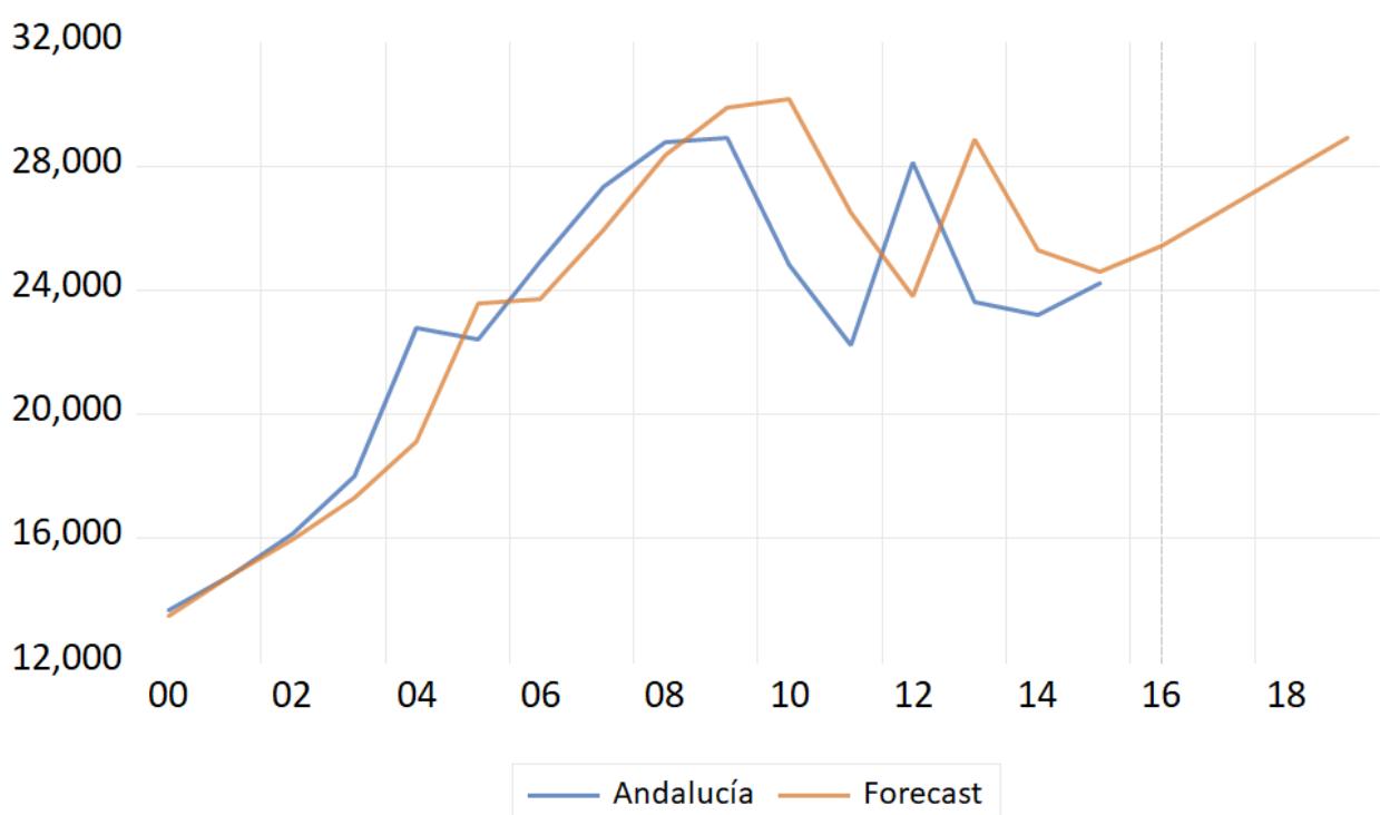
2. Aragón
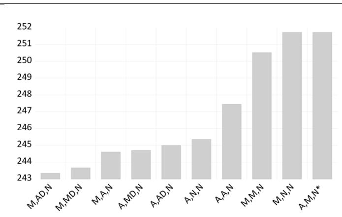
| Parameters | |
| Alpha (fixed): | 0.900000 |
| Beta: | 0.000000 |
| Phi: | 0.853986 |
Initial Parameters
| Initial level: | 826.5191 |
| Initial trend: | 836.3896 |
| Compact Log-likelihood | -118.6654 |
| Log-likelihood | -119.1877 |
| Akaike Information Criterion | 243.3309 |
| Schwarz Criterion | 245.6486 |
| Hannan-Quinn Criterion | 243.4496 |
| Sum of Squared Residuals | 0.194730 |
| Root Mean Squared Error | 0.110321 |
| Average Mean Squared Error | 255309.2 |
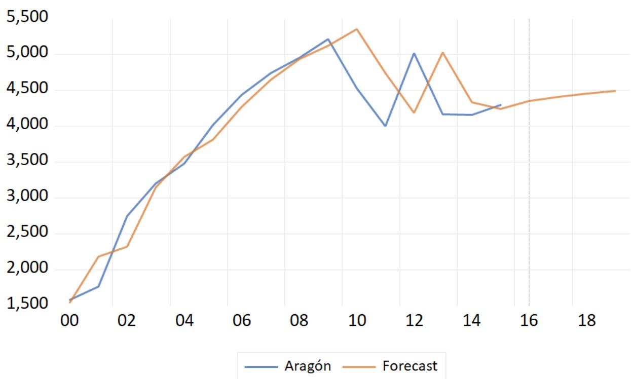
3. Principado de Asturias
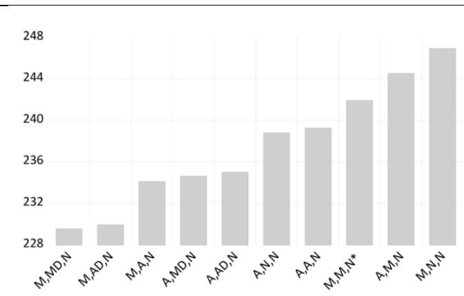
ETS Smoothing Original series: PRINCIPADO_DE_ASTURIAS Date: 10/13/25 Time: 16:32 Sample: 2000 2019 Included observations: 16 Model: M,MD,N - Multiplicative Error, Multiplicative -Dampened Trend, No Season (Auto E=*, T= *) Model selection: Akaike Information Criterion Convergence achieved after 0 iterations
| Parameters | |
| Alpha (fixed): | 0.900000 |
| Beta: | 0.000000 |
| Phi: | 0.678701 |
Initial Parameters
| Initial level: | 711.7421 |
| Initial trend: | 2.296837 |
| Compact Log-likelihood | -111.7755 |
| Log-likelihood | -112.2978 |
| Akaike Information Criterion | 229.5510 |
| Schwarz Criterion | 231.8688 |
| Hannan-Quinn Criterion | 229.6697 |
| Sum of Squared Residuals | 0.108899 |
| Root Mean Squared Error | 0.082499 |
| Average Mean Squared Error | 146637.2 |
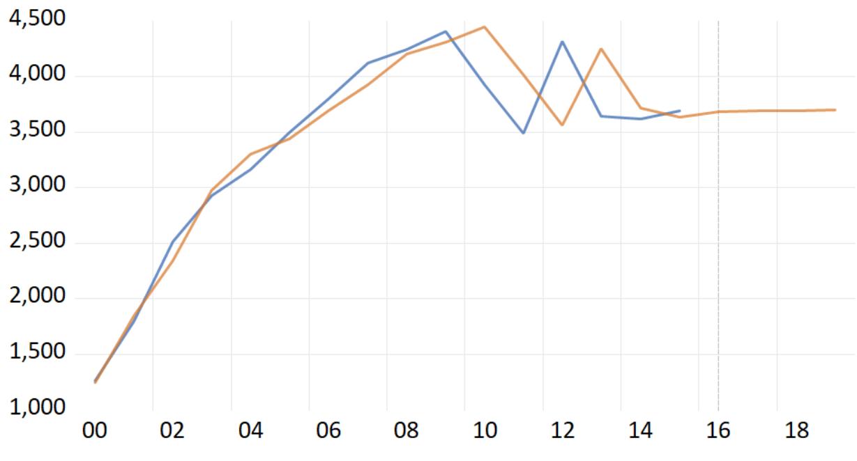
Principado de Asturias — Forecast
| Parameters | |
| Alpha (fixed): | 0.900000 |
| Beta: | 0.000000 |
| Initial Parameters | |
| Initial level: | 669.8659 |
| Initial trend: | 312.1365 |
| Compact Log-likelihood | -117.5232 |
| Log-likelihood | -118.0455 |
| Akaike Information Criterion | 239.0464 |
| Schwarz Criterion | 240.5915 |
| Hannan-Quinn Criterion | 239.1255 |
| Sum of Squared Residuals | 0.310760 |
| Root Mean Squared Error | 0.139365 |
| Average Mean Squared Error | 260297.5 |
4. Baleares
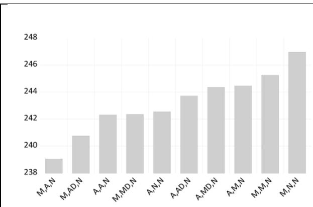
ETS Smoothing Original series: BALEARES Date: 10/13/25 Time: 16:48 Sample: 2000 2019 Included observations: 16 Model: M,A,N - Multiplicative Error, Additive Trend, No Season (Auto E=*, T=*) Model selection: Akaike Information Criterion Convergence achieved after 1 iteration
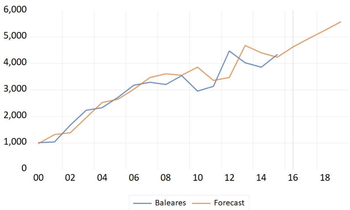
5. Canarias
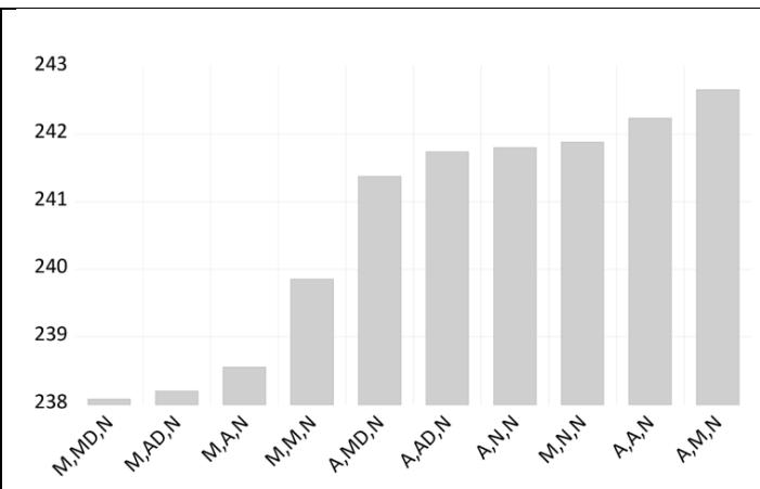
ETS Smoothing Original series: CANARIAS Date: 10/13/25 Time: 16:05 Sample: 2000 2019 Included observations: 16 Model: M.MD.N - Multiplicative Error, Multiplicative -Dampened Trend, No Season (Auto E=*, T= *) Model selection: Akaike Information Criterion Convergence achieved after 1 iteration
| Parameters | |
| Alpha (fixed): | 0.900000 |
| Beta: | 0.000000 |
| Phi: | 0.829306 |
Initial Parameters
| Initial parameters | |
| Initial level: | 4084.363 |
| Initial trend: | 1.155564 |
| Compact Log-likelihood | -116.0376 |
| Log-likelihood | -116.5599 |
| Akaike Information Criterion | 238.0752 |
| Schwarz Criterion | 240.3929 |
| Hannan-Quinn Criterion | 238.1938 |
| Sum of Squared Residuals | 0.044013 |
| Root Mean Squared Error | 0.052448 |
| Average Mean Squared Error | 355027.6 |
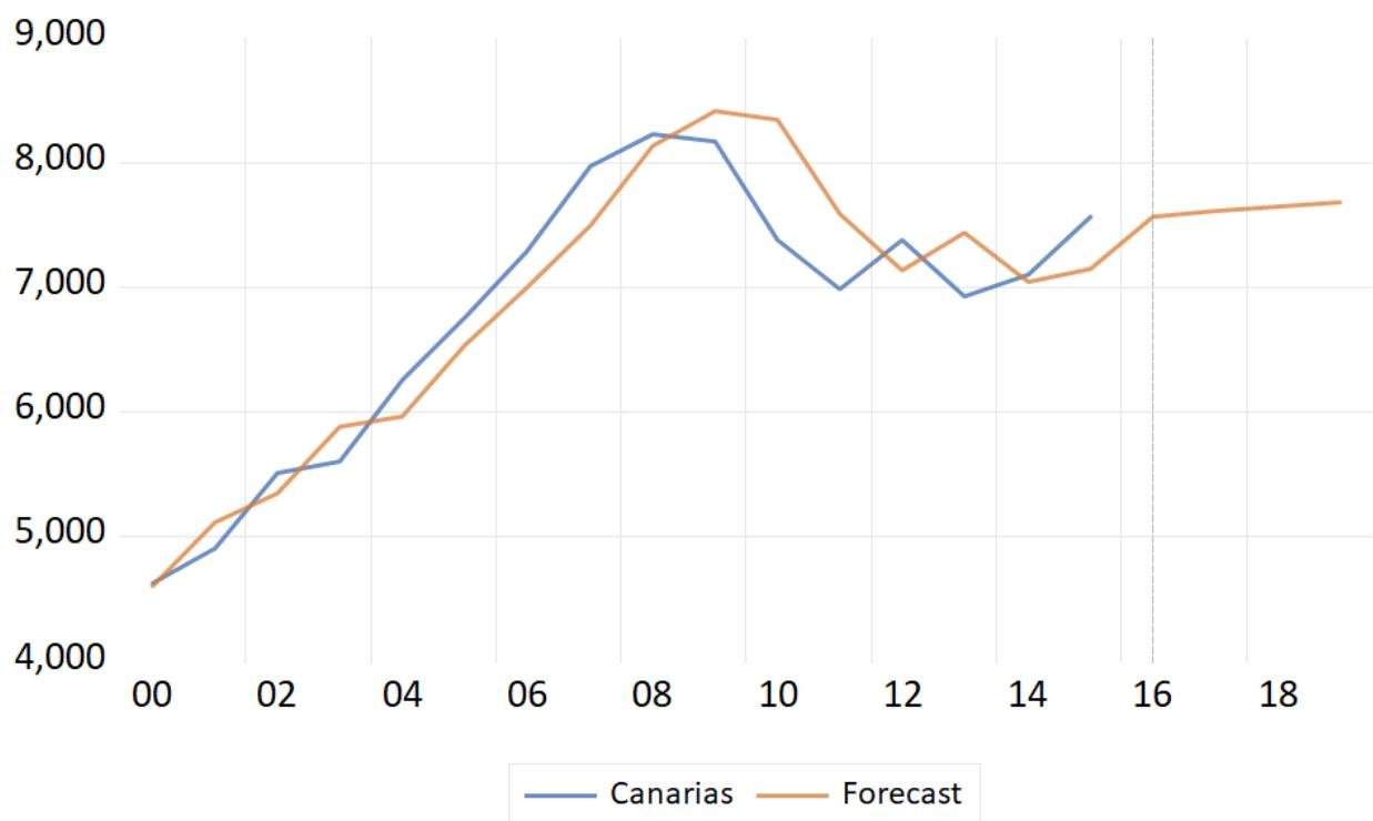
Cantabria Forecast
6. Cantabria
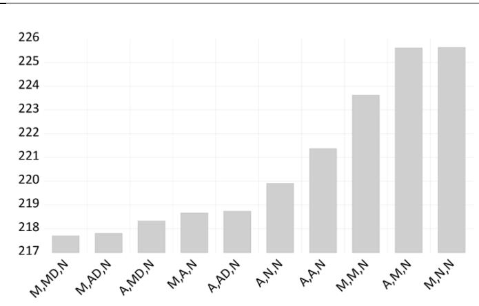
ETS Smoothing Original series: CANTABRIA Date: 10/13/25 Time: 16:06 Sample: 2000 2019 Included observations: 16 Model: M,MD,N - Multiplicative Error, Multiplicative -Dampened Trend, No Season (Auto E=*, T= *)
| Parameters | |
| Alpha (fixed): | 0.900000 |
| Beta: | 0.000000 |
| Phi: | 0.774979 |
Initial Parameters
| Initial level: | 588.7950 |
| Initial trend: | 1.562154 |
| Compact Log-likelihood | -105.8494 |
| Log-likelihood | -106.3717 |
| Akaike Information Criterion | 217.6989 |
| Schwarz Criterion | 220.0166 |
| Hannan-Quinn Criterion | 217.8176 |
| Sum of Squared Residuals | 0.155346 |
| Root Mean Squared Error | 0.098535 |
| Average Mean Squared Error | 59951.15 |
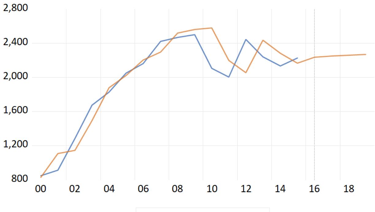
7. Cataluña
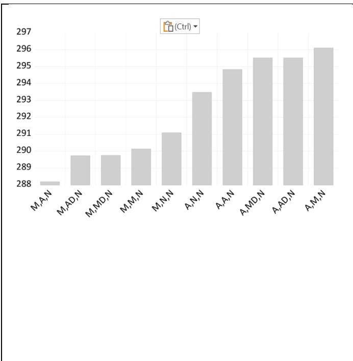
ETS Smoothing Original series: CATALUNA Date: 10/13/25 Time: 16:10 Sample: 2000 2019 Included observations: 16 Model: M,A,N - Multiplicative Error, Additive Trend No Season (Auto E=*, T=*) Model selection: Akaike Information Criterion Convergence achieved after 1 iteration
| Parameters | |
| Alpha (fixed): | 0.900000 |
| Beta: | 0.000000 |
| Initial Parameters | |
| Initial level: | 11236.73 |
| Initial trend: | 1180.102 |
| Compact Log-likelihood | -142.0944 |
| Log-likelihood | -142.6167 |
| Akaike Information Criterion | 288.1888 |
| Schwarz Criterion | 289.7340 |
| Hannan-Quinn Criterion | 288.2679 |
| Sum of Squared Residuals | 0.113631 |
| Root Mean Squared Error | 0.084273 |
| Average Mean Squared Error | 7019195. |
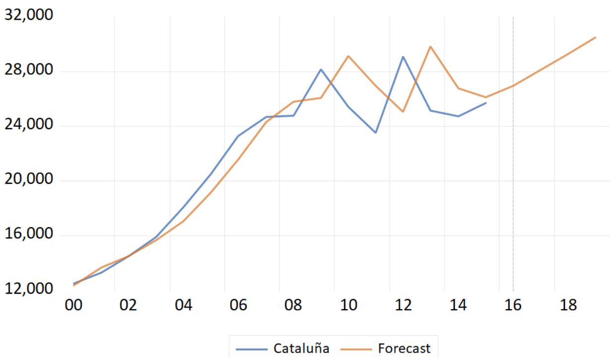
8. Castilla-La Mancha
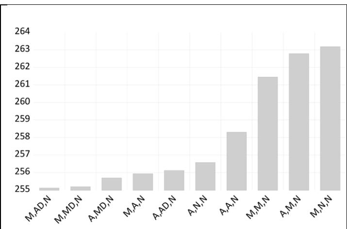
ETS Smoothing Original series: CASTILLA_LA_MANCHA Date: 10/13/25 Time: 16:08 Sample: 2000 2019 Included observations: 16 Model: M,AD,N - Multiplicative Error, Additive -Dampened Trend, No Season (Auto E=*, T= *)
| Parameters | |
| Alpha (fixed): | 0.900000 |
| Beta: | 0.000000 |
| Phi: | 0.862907 |
Initial Parameters
| Initial level: | 1183.142 |
| Initial trend: | 1129.529 |
| Compact Log-likelihood | -124.5589 |
| Log-likelihood | -125.0812 |
| Akaike Information Criterion | 255.1178 |
| Schwarz Criterion | 257.4355 |
| Hannan-Quinn Criterion | 255.2364 |
| Sum of Squared Residuals | 0.200816 |
| Root Mean Squared Error | 0.112031 |
| Average Mean Squared Error | 572780.9 |
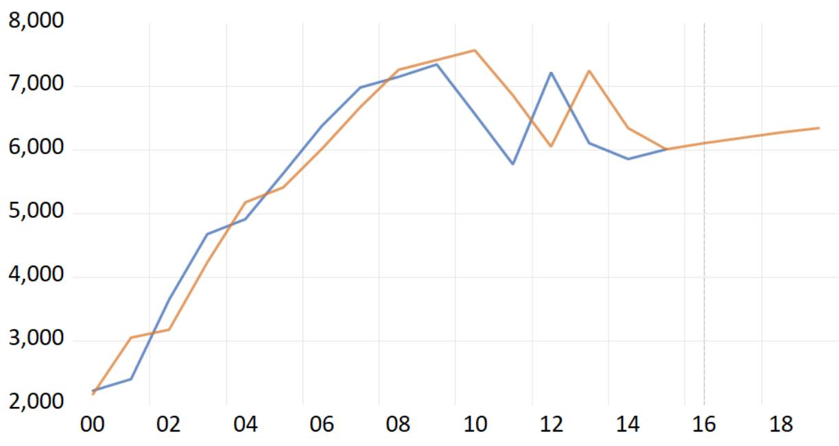
- Castilla-La Mancha Forecast
9. Castilla y León
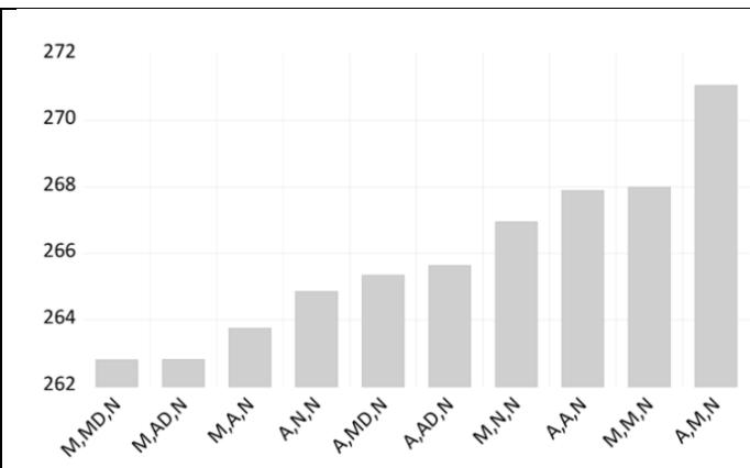
ETS Smoothing Original series: CASTILLA_Y_LEON Date: 10/13/25 Time: 16:09 Sample: 2000 2019 Included observations: 16 Model: M,MD,N - Multiplicative Error, Multiplicative -Dampened Trend, No Season (Auto E=*, T= *) Model selection: Akaike Information Criterion Convergence achieved after 1 iteration
| Parameters | |
| Alpha (fixed): | 0.900000 |
| Beta: | 0.000000 |
| Phi: | 0.768905 |
Initial Parameters
| Initial level: | 2801.680 |
| Initial trend: | 1.455941 |
| Compact Log-likelihood | -128.4008 |
| Log-likelihood | -128.9231 |
| Akaike Information Criterion | 262.8017 |
| Schwarz Criterion | 265.1194 |
| Hannan-Quinn Criterion | 262.9204 |
| Sum of Squared Residuals | 0.165362 |
| Root Mean Squared Error | 0.101662 |
| Average Mean Squared Error | 838723.7 |
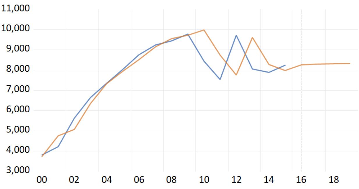
Castilla y León Forecast
10. Extremadura
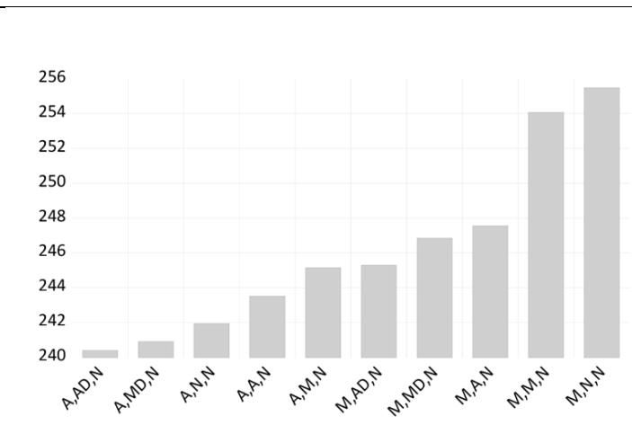
ETS Smoothing Original series: EXTREMADURA Date: 10/13/25 Time: 16:20 Sample: 2000 2019 Included observations: 16 Model: A.AD,N - Additive Error, Additive-Dampened Trend, No Season (Auto E=*, T=*) Model selection: Akaike Information Criterion Convergence achieved after 0 iterations
| Parameters | |
| Alpha (fixed): | 0.900000 |
| Beta: | 0.000000 |
| Phi: | 0.789936 |
Initial Parameters
| Initial level: | 649.5925 |
| Initial trend: | 1066.815 |
| Compact Log-likelihood | -117.1924 |
| Log-likelihood | -117.7147 |
| Akaike Information Criterion | 240.3847 |
| Schwarz Criterion | 242.7025 |
| Hannan-Quinn Criterion | 240.5034 |
| Sum of Squared Residuals | 2301442. |
| Root Mean Squared Error | 379.2626 |
| Average Mean Squared Error | 156005.4 |
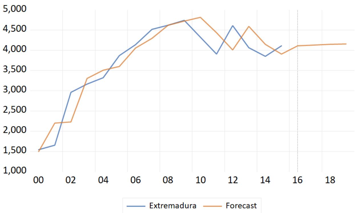
11. Galicia
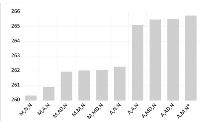
ETS Smoothing Original series: GALICIA Date: 10/13/25 Time: 16:27 Sample: 2000 2019 Included observations: 16 Model: M,AD,N - Multiplicative Error, Additive -Dampened Trend, No Season Convergence achieved after 1 iteration
| Parameters | |
| Alpha (fixed): | 0.900000 |
| Beta: | 0.000000 |
| Phi: | 0.893393 |
Initial Parameters
| Initial level: | 5211.410 |
| Initial trend: | 753.7447 |
| Compact Log-likelihood | -127.9677 |
| Log-likelihood | -128.4900 |
| Akaike Information Criterion | 261.9353 |
| Schwarz Criterion | 264.2531 |
| Hannan-Quinn Criterion | 262.0540 |
| Sum of Squared Residuals | 0.116508 |
| Root Mean Squared Error | 0.085333 |
| Average Mean Squared Error | 1021414. |
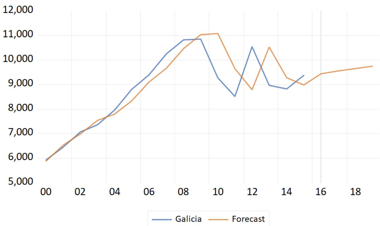
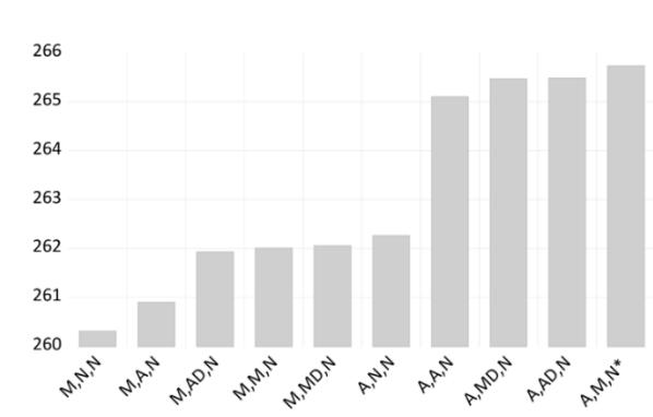
ETS Smoothing Original series: GALICIA Date: 10/13/25 Time: 16:29 Sample: 2000 2019 Included observations: 16 Model: M,N,N - Multiplicative Error, No Trend, No Season (Auto E=*, T=*) Model selection: Akaike Information Criterion Convergence achieved after 5 iterations
| Parameters | |
| Alpha (fixed): | 0.900000 |
| Initial Parameters | |
| Initial level: | 5931.776 |
| Compact Log-likelihood | -130.1577 |
| Log-likelihood | -130.6800 |
| Akaike Information Criterion | 260.3153 |
| Schwarz Criterion | 260.3153 |
| Hannan-Quinn Criterion | 260.3153 |
| Sum of Squared Residuals | 0.165549 |
| Root Mean Squared Error | 0.101719 |
| Average Mean Squared Error | 1463261. |
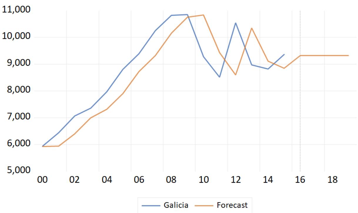
12. La Rioja
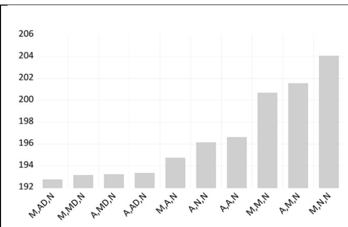
ETS Smoothing Original series: LA_RIOJA Date: 10/13/25 Time: 16:30 Sample: 2000 2019 Included observations: 16 Model: M,AD.N - Multiplicative Error, Additive -Dampened Trend. No Season (Auto E=*. T= *) Model selection: Akaike Information Criterion Convergence achieved after 0 iterations
| Parameters | |
| Alpha (fixed): | 0.900000 |
| Beta: | 0.000000 |
| Phi: | 0.850468 |
| Initial Parameters | |
| Initial level: | 231.5440 |
| Initial trend: | 208.8311 |
| Compact Log-likelihood | -93.36820 |
| Log-likelihood | -93.89051 |
| Akaike Information Criterion | 192.7364 |
| Schwarz Criterion | 195.0542 |
| Hannan-Quinn Criterion | 192.8551 |
| Sum of Squared Residuals | 0.128588 |
| Root Mean Squared Error | 0.089648 |
| Average Mean Squared Error | 10256.77 |
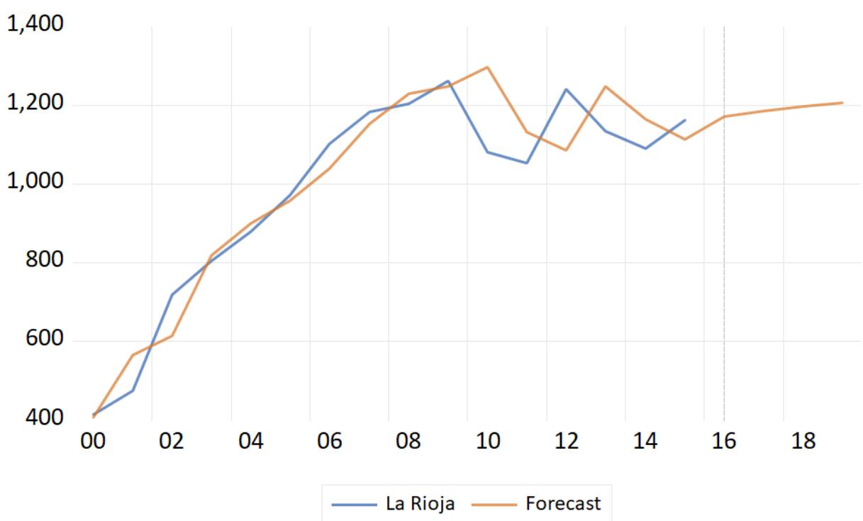
13. Comunidad de Madrid
Comunidad de Madrid Forecast
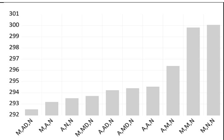
ETS Smoothing Original series: COMUNIDAD DE MADRID Date: 10/13/25 Time: 16:12 Sample: 2000 2019 Included observations: 16 Model: M,AD.N - Multiplicative Error, Additive -Dampened Trend, No Season (Auto E=*. T= *)
| Parameters | |
| Alpha (fixed): | 0.900000 |
| Beta: | 0.000000 |
| Phi: | 0.880050 |
Initial Parameters
| Initial level: | 3645.755 |
| Initial trend: | 3210.285 |
| Compact Log-likelihood | -143.2541 |
| Log-likelihood | -143.7764 |
| Akaike Information Criterion | 292.5082 |
| Schwarz Criterion | 294.8260 |
| Hannan-Quinn Criterion | 292.6269 |
| Sum of Squared Residuals | 0.232511 |
| Root Mean Squared Error | 0.120548 |
| Average Mean Squared Error | 4484740. |
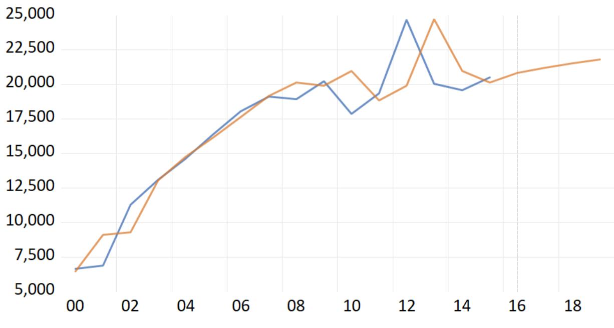
14. Región de Murcia
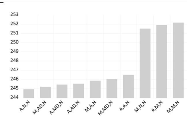
ETS Smoothing Original series: REGION_DE_MURCIA Date: 10/13/25 Time: 16:36 Sample: 2000 2019 Included observations: 16 Model: M,AD.N - Multiplicative Error, Additive -Dampened Trend, No Season Convergence achieved after 0 iterations
| Parameters | |
| Alpha (fixed): | 0.900000 |
| Beta: | 0.000000 |
| Phi: | 0.875994 |
Initial Parameters
| Initial level: | 849.6975 |
| Initial trend: | 716.1437 |
| Compact Log-likelihood | -119.5953 |
| Log-likelihood | -120.1176 |
| Akaike Information Criterion | 245.1907 |
| Schwarz Criterion | 247.5084 |
| Hannan-Quinn Criterion | 245.3093 |
| Sum of Squared Residuals | 0.244783 |
| Root Mean Squared Error | 0.123689 |
| Average Mean Squared Error | 262797.3 |
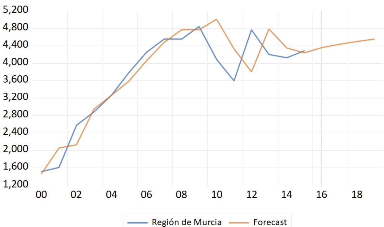
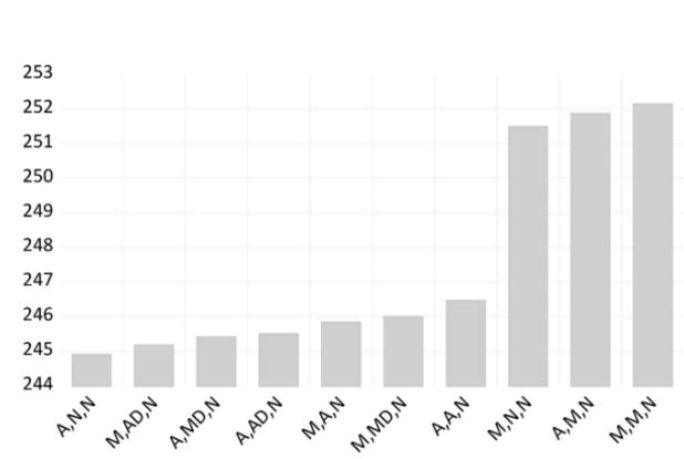
ETS Smoothing Original series: REGION_DE MURCIA Date: 10/13/25 Time: 16:34 Sample: 2000 2019 Included observations: 16 Model: A.N.N - Additive Error, No Trend. No Season (Simple exponential model) (Auto E=*. T=*) Model selection: Akaike Information Criterion Convergence achieved after 3 iterations
| Parameters | |
| Alpha (fixed): | 0.900000 |
| Initial Parameters | |
| Initial level: | 1535.323 |
| Compact Log-likelihood | -122.4595 |
| Log-likelihood | -122.9818 |
| Akaike Information Criterion | 244.9190 |
| Schwarz Criterion | 244.9190 |
| Hannan-Quinn Criterion | 244.9190 |
| Sum of Squared Residuals | 4445645. |
| Root Mean Squared Error | 527.1174 |
| Average Mean Squared Error | 564304.1 |
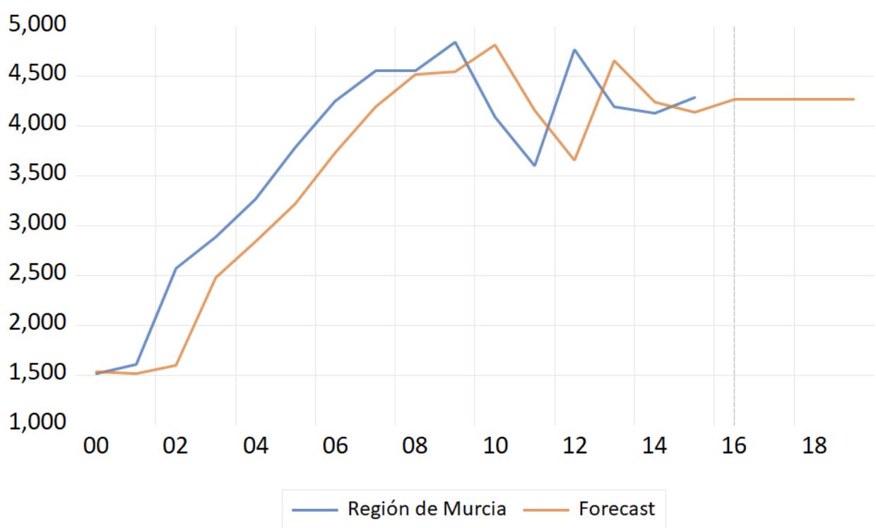
15. Navarra
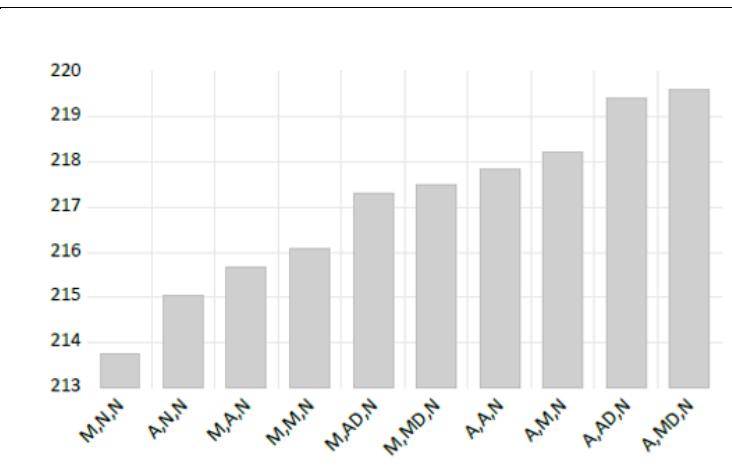
ETS Smoothing Original series: COMUNIDAD_FORAL_DE_NAVA Date: 10/13/25 Time: 16:15 Sample: 2000 2019 Included observations: 16 Model: M,MD,N - Multiplicative Error, Multiplicative -Dampened Trend, No Season (Auto E=*) Model selection: Akaike Information Criterion Convergence achieved after 1 iteration
| Parameters | |
| Alpha (fixed): | 0.900000 |
| Beta: | 0.000000 |
| Phi: | 0.899699 |
| Initial Parameters | |
| Initial level: | 2619.334 |
| Initial trend: | 1.045894 |
| Compact Log-likelihood | -105.7442 |
| Log-likelihood | -106.2665 |
| Akaike Information Criterion | 217.4884 |
| Schwarz Criterion | 219.8062 |
| Hannan-Quinn Criterion | 217.6071 |
| Sum of Squared Residuals | 0.052072 |
| Root Mean Squared Error | 0.057048 |
| Average Mean Squared Error | 102951.6 |
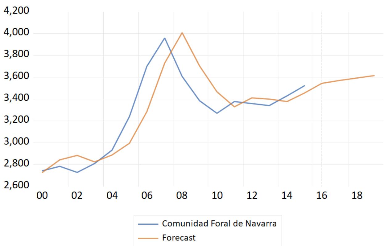
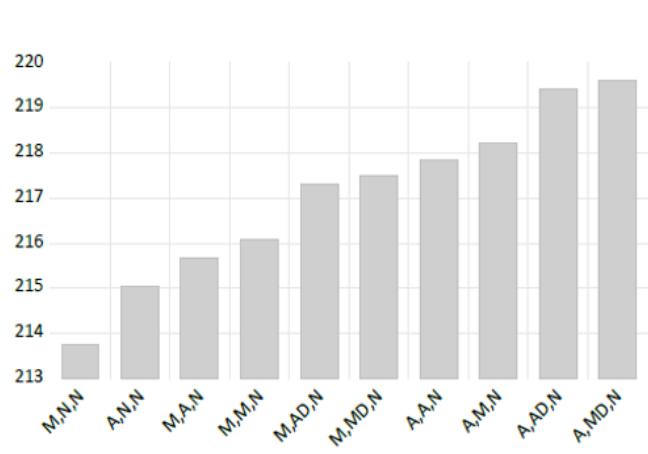
ETS Smoothing Original series: COMUNIDAD FORAL DE NAVARRA Date: 02/26/26 Time: 11:08 Sample: 2000 2019 Included observations: 16 Model: M,N,N - Multiplicative Error, No Trend, No Season (Auto E=*, T=*) Model selection: Akaike Information Criterion Convergence achieved after 4 iterations
| Parameters | |
| Alpha (fixed): | 0.900000 |
| Initial Parameters | |
| Initial level: | 2735.897 |
| Compact Log-likelihood | -106.8706 |
| Log-likelihood | -107.3929 |
| Akaike Information Criterion | 213.7412 |
| Schwarz Criterion | 213.7412 |
| Hannan-Quinn Criterion | 213.7412 |
| Sum of Squared Residuals | 0.062353 |
| Root Mean Squared Error | 0.062426 |
| Average Mean Squared Error | 115357.7 |
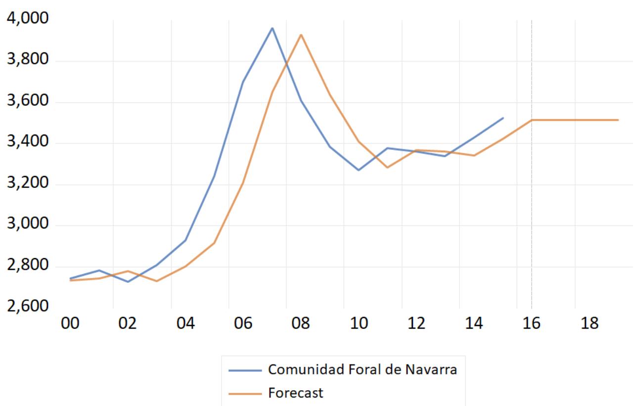
| Parameters | |
| Alpha (fixed): | 0.900000 |
| Beta: | 0.000000 |
| Initial Parameters | |
| Initial level: | 5295.186 |
| Initial trend: | 308.0540 |
| Compact Log-likelihood | -119.6876 |
| Log-likelihood | -120.2099 |
| Akaike Information Criterion | 243.3753 |
| Schwarz Criterion | 244.9204 |
| Hannan-Quinn Criterion | 243.4544 |
| Sum of Squared Residuals | 0.049176 |
| Root Mean Squared Error | 0.055439 |
| Average Mean Squared Error | 512498.0 |
16. País Vasco
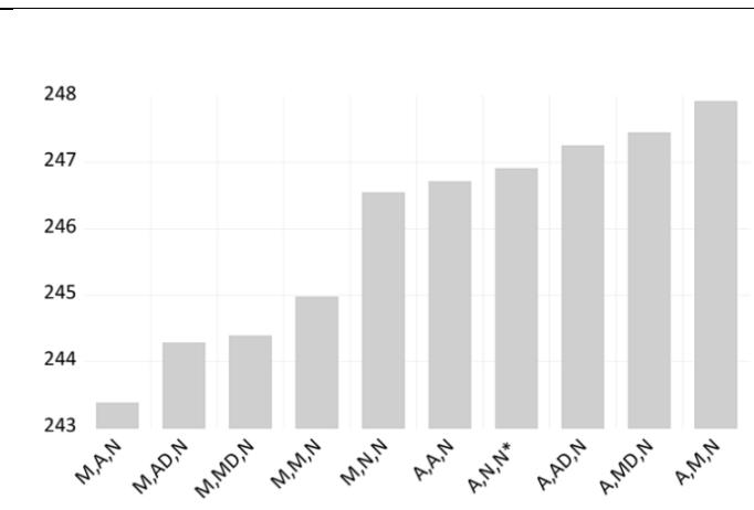
ETS Smoothing Original series: PAIS_VASCO Date: 10/13/25 Time: 16:31 Sample: 2000 2019 Included observations: 16 Model: M,A,N - Multiplicative Error, Additive Trend No Season (Auto E=*, T=*) Model selection: Akaike Information Criterion Convergence achieved after 1 iteration
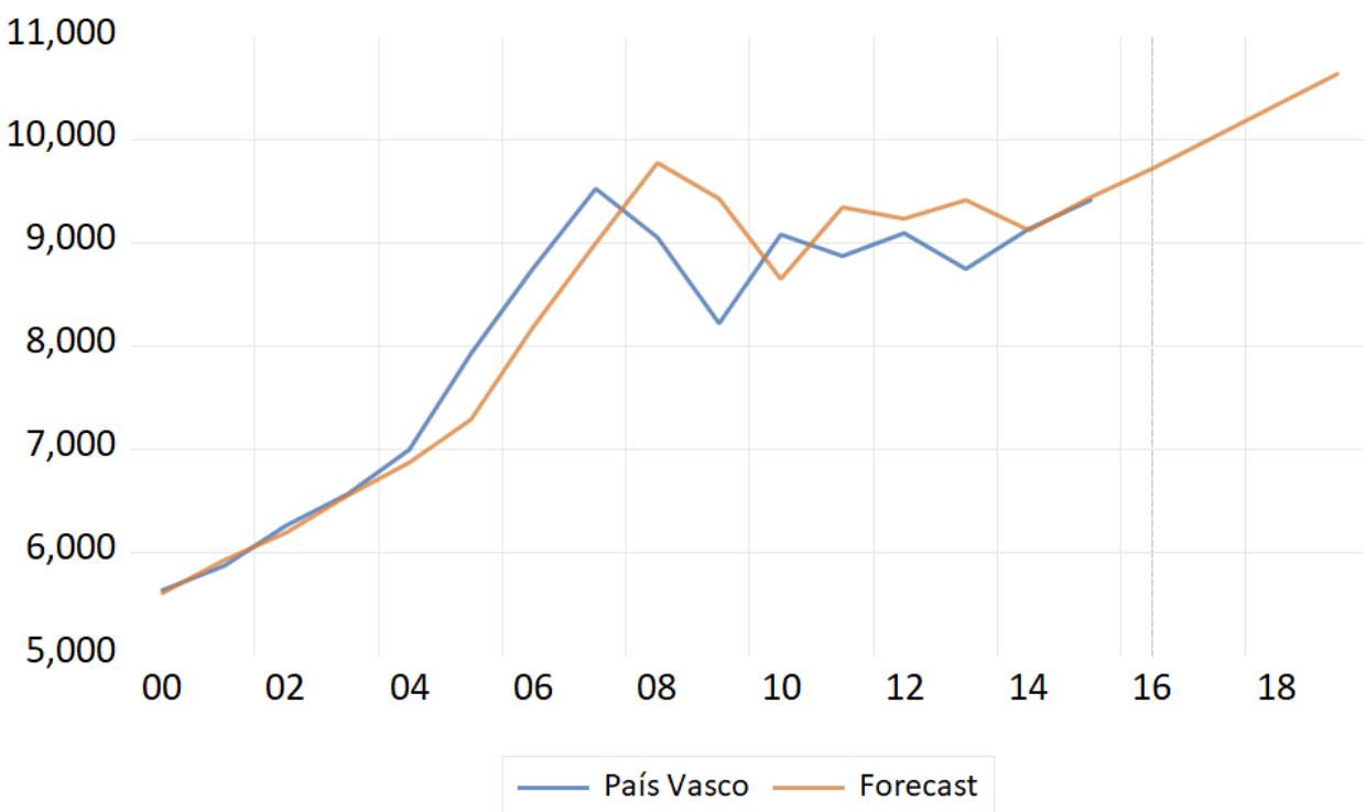
17. Comunitat Valenciana
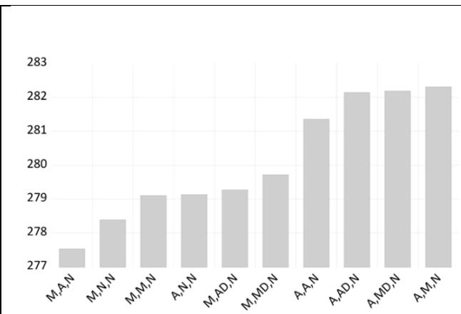
ETS Smoothing Original series: COMUNITAT_VALENCIA Date: 10/13/25 Time: 16:18 Sample: 2000 2019 Included observations: 16 Model: M,A,N - Multiplicative Error, Additive Trend, No Season (Auto E=*, T=*) Model selection: Akaike Information Criterion Convergence achieved after 1 iteration
| Parameters | |
| Alpha (fixed): | 0.900000 |
| Beta: | 0.000000 |
Initial Parameters
| Initial level: | 6627.131 |
| Initial trend: | 691.9034 |
| Compact Log-likelihood | -136.7662 |
| Log-likelihood | -137.2885 |
| Akaike Information Criterion | 277.5323 |
| Schwarz Criterion | 279.0775 |
| Hannan-Quinn Criterion | 277.6115 |
| Sum of Squared Residuals | 0.174417 |
| Root Mean Squared Error | 0.104408 |
| Average Mean Squared Error | 3214953. |
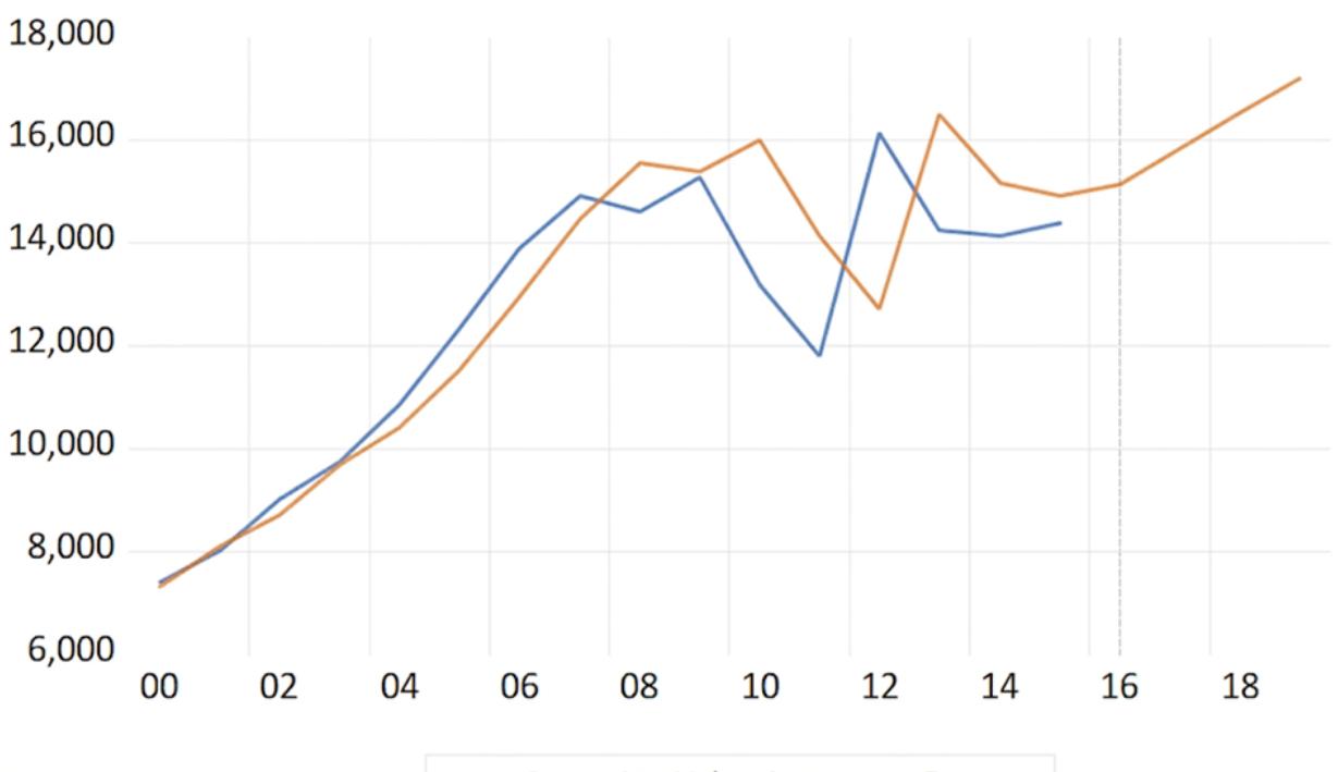
Comunitat Valenciana Forecast
Este texto se ha extraído automáticamente del documento original. Para citarlo o leerlo con su maquetación, descargue el PDF.
Descargar en PDF