Replacement investment, endogenous fluctuations and the dynamics of job creation and job destruction by Raouf Boucekkine* Fernando del Río* Omar Licandro**

DOCUMENTO DE TRABAJO 97-13

Julio, 1997

* Universidad Carlos III de Madrid. ** FEDEA and Universidad Carlos III de Madrid.

Raouf Boucekkine Universidad Carlos III

Fernando del Río Universidad Carlos III

Omar Licandro FEDEA and Universidad Carlos III

July 2, 1997

Abstract

In this paper, we present a basic framework for the discussion of the controversial dynamic properties of job creation and job destruction. To this end, we consider a simplified version of Caballero and Hammour's creative destruction model (1996). In particular, we remove the exogenous fluctuations source of this model and we assume that the marginal hiring cost is constant. This allows us at first to solve explicitly for the dynamics of the model. We show that the optimal lifetime of capital goods is constant at the decentralized equilibrium and we prove that the hiring and firing rates convergence to their steady state growth paths values is oscillatory, due to endogenous replacement echoes. We find that when business fluctuations are endogenous, job creation is smoother than job destruction even if the marginal hiring cost is constant. Moreover, depending on the initial job profile, we show that job creation can be either positively or negatively correlated with job destruction.

Keywords: Creative destruction, Job creation and destruction, Endogenous fluctuations, Differential-difference equations.

Journal of Economic Literature: E22, E32, O40, C63.

*Correspondence: R. Boucekkine, Universidad Carlos III de Madrid, Departamento de Economía, Calle Madrid 126, 28903 Getafe (Madrid), Spain. E-Mail: barouf@eco.uc3m.es

1 Introduction

In the recent years, many empirical studies have enhanced the role of gross flows of workers (into and out employment, unemployment and the labor force) in the dynamics of the labor market. A key question turns out to be whether these flows are the result of a creative destruction process of job opportunities. By a creative destruction process, we refer to the Schumpeterian view that associates economic growth and technical progress with a continuous structural change involving the “death” of some productive activities (with the resulting destroyed jobs) and their replacement by more efficient activities (with the resulting created jobs). The results reported by Davis and Haltiwanger (1990, 1992) for the US economy have reinforced the latter interpretation. Precisely, these authors find that around 35 percents of gross flows of workers into and out employment and unemployment are due to creative destruction.

Creative destruction has been recently deeply analyzed in the economic literature . In this literature, technical progress is exclusively embodied in the new capital goods. Nowadays, it is generally admitted that a large part of technical progress is embodied. Although there is still a controversy concerning the quantitative importance of embodiment as a source of economic growth (see Hulten (1992) for details on this controversy), many authors have emphasized the role of embodied technical change in the explanation of a number of fundamental macroeconomic and microeconomic stylized facts (see Cooley et al (1994) and Doms et al (1995) for example). Once technical progress is embodied in the new capital goods, the older equipments become less and less profitable over time and may be substituted by these new capital goods. The vintage capital growth models are obviously more suitable to deal with this process. Note however that not all vintage capital growth models generate an endogenous process of creative destruction. The key assumption in this respect is the substituability between labor and capital. If gross substituability is allowed, it may be optimal to never scrap any machine whatever is its age (No destruction). Rather, the optimal decision would be to reduce the number of workers operating the oldest machines over time but to never throw them out at a finite date (See Benhabib and Rustichini (1993)). Therefore, if one aims at theoretically investigating job creation and destruction in line with the Schumpeterian view, one should impose factor complementarity or add some non-trivial specifications to ensure finite time scrapping under substituability. As most of the recent contributions in the topic, we assume a Leontieff technology.

The empirical literature in the topic has focused on the cyclical properties of job creation, destruction and reallocation. Most of these empirical studies conducted on different national economies datas find that job creation is procyclical and that job destruction is counter-cyclical. However, the cyclical properties of job reallocation, the sum of job creation and job destruction, are controversial. Indeed, job reallocation is counter-cyclical on US data (Davis Haltiwanger (1992, 1994)) and on UK data (Konings (1995)), whereas it appears acyclical on Spanish data (Dolado and Gómez (1995)) or on German data (Boeri and Cramer (1991)). It is worth pointing out that the counter-cyclicity of job reallocation is highly consistent with the theories claiming that it is more efficient to concentrate job reallocation during recessions (see the cleansing effects of recessions view exposed in Caballero and Hammour (1994)). During recessions, the opportunity cost of generating unemployment is typically low and this should incentivate job creation as well as job destruction. As a consequence, job creation and destruction should increase together during a recession, which implies that job creation, job destruction and job reallocation should be positively correlated. The empirical results reported above show that the latter prediction is not checked in the real world. Moreover, most empirical studies (see for example Davis and Haltiwanger (1990, 1992)) have found that job creation and job destruction are not synchronized in many respects: As a matter of fact, job destruction appears to be much higher than creation during recessions, job creation being markedly smoother than job destruction.

See in particular Aghion and Howitt (1992,1994) and Caballero and Hammour (1994,1996).

These non-synchronization features (or decoupling) have been recently theoretically analyzed by Caballero and Hammour (1996). The authors show how decoupling can result from the existence of inefficient decentralized equilibria. Assuming a general structure for hiring costs, they consider a labor market in which workers and a representative firm bargain over an appropriable surplus. This appropriability problem introduces a kind of wage rigidity which makes the decentralized equilibrium inefficient and causes the non-synchronization between job creation and destruction. Moreover, depending on the structure of the hiring costs, the authors are able to generate different job creation and destruction behaviours in terms of synchronization and volatility. In particular, when the marginal creation cost is increasing with respect to job creation, job creation is smooth and negatively correlated with job destruction at the (inefficient) decentralized equilibrium, as reported in the empirical literature.

In this paper, we assume that the marginal job creation cost is constant and we analyze the implications of another determinant of job creation dynamics. Using a simplified version of Caballero and Hammour's model (1996), we focus on the consequences of purely endogenous replacement investment activity on the dynamics of job creation and job destruction, in contrast to Caballero and Hammour's model where business fluctuations are driven by exogenous profitability cycles. To this end, we remove the exogenous price of the non-produced good of the latter model, which precisely causes the profitability cycles. Thus, fluctuations are purely endogenous in our setting according to echo effects (see Benhabib and Rustichini (1991, 1993) and Boucekkine et al. (1997-a)). Creative destruction consists principally in a replacement investment activity and this may generate a strong correlation between the current cycle and the previous cycles. Indeed, echo effects do occur even in the general model solved by Caballero and Hammour, as recognized by these authors themselves (footnote 19, page 820). However, for certain specifications of this model and for certain magnitudes of its exogenous cycles, the exogenous fluctuations will dominate echo effects. This raises two questions. It is likely that Caballero and Hammour have parameterized their model, and in particular the characteristics of the exogenous cycles, in such a way that the impact of echo effects is minimized. What would happen in models where the exogenous cycles are not strong enough to offset the effects of the endogenous replacement activity? This is an interesting theoretical question that we tackle here by analyzing the extreme case where fluctuations are solely caused by endogenous replacement investment. The other question concerns the synchronization between job creation and job destruction in the absence of any exogenously driven fluctuations. Caballero and Hammour (1996) have focused on the structure of the job creation cost to generate the different dynamic behaviours of job creation and destruction, and have concluded that an increasing marginal cost allows to replicate some of the major stylized facts reported in the empirical literature. In this paper, we assume that this marginal cost is constant. This allows us to solve the model explicitly and more importantly, it ultimately allows us to point at another economic factor that is likely to matter in the dynamics of job reallocation, namely the initial profile of jobs. In particular, even if the marginal cost of job creation is constant, our simple model can generate a smooth job creation, a volatile job destruction and a negative correlation between these two variables as in the real world. Obviously, we do not argue here that the fluctuations due to the endogenous replacement investment activity are the major determinant of the dynamics of job creation and destruction. However, we do think that the “historical” conditions in the labor market can be a relevant determinant in certain real world cases. For example, some economists have argued that the low level of job reallocation in the UK during the period 1985-91 is due to the anterior intensive industrial restructuring that took place during the first years of Mrs Thatcher’s government (see Konings (1995) for example).

As stressed above, we solve our model explicitly in sharp contrast to the existing related theoretical literature which mostly uses numerical simulation techniques (as in Caballero and Hammour (1994, 1996)) or even is restricted to the analysis of the stationary equilibria (as in Aghion and Howitt (1994)). The paper is organized as follows. Section 2 describes our model as a particular case of Caballero and Hammour's model (1996). Section 3 gives the analytical resolution of the model and its short run dynamics. In Section 4, we study the asymptotic stability of the model and we shed light on the synchronization properties between job creation and destruction when fluctuations are purely endogenous. Section 5 concludes.

2 The Economy

As stated in the introduction, our main deviation with respect to Caballero and Hammour's (CH hereafter) model (1996) resides in the fact that we remove the intermediate good sector which exogenous price fluctuations cause the profitability cycles in this model. We consider a one sector model in which the production technology is the usual Leontieff vintage capital technology with exogenous (Harrod neutral) labor augmenting technical progress (see Solow et al (1966)). Technical progress is continuously embodied in the new capital goods, which yields an endogenous process of creation and destruction through the replacement of the old obsolescent machines by the new (more productive) capital goods. We assume that technological progress is exponential such that labor productivity grows exogenously at rate . The Leontieff technology described below states that a capital unit of vintage t requires an amount of labor equal to to be operated, and produces one unit of output.

If we denote by the age of the oldest operating machines at time t (or alternatively the age of the oldest filled job), aggregate employment and output are given by

\[y (t) = \int_ {t - T (t)} ^ {t} e ^ {\gamma \tau} h (\tau) d \tau ,\tag{1}\]

and

\[l (t) = \int_ {t - T (t)} ^ {t} h (\tau) d \tau .\tag{2}\]

is the amount of labor devoted to operate machines of vintage t. It can be interpreted as the creation of employment at time t.

Another simplifying assumption with respect to CH concerns the structure of the cost of job creation. In CH's paper, this cost depends upon the number of created jobs and on the unemployment rate, the marginal creation cost being consequently state-dependent. In this paper, we assume that the marginal cost of job creation is constant in order to characterize explicitly the dynamics of the model. This assumption is perfectly consistent with the objectives of this paper. It is clear that the structure of the hiring cost does matter in the dynamics of job creation and destruction. However, this paper aims at putting forward the role of endogenous replacement echoes in the latter dynamics. Because replacement echoes are likely to occur independently of the cost structure (as it can be inferred from CH's work), the constant marginal cost assumption actually allows to analyze somewhat separately the dynamic properties of job creation and destruction due to the sole replacement echoes. Concretely, we assume that the firm has a unit hiring cost with a positive real number. Additionally, as in any Leontieff model, a job creation requires an investment cost: Creating a job requires the installation of units of capital.

The model is completed by the specification of consumer preferences and by a job search process as in CH. The economy comprises a continuum of agents, indexed from 0 to 1, with the same linear preferences over lifetime consumption:

\[\int_ {0} ^ {\infty} c (\tau) e ^ {- r \tau} d \tau ,\]

where is the subjective rate of time preference, and is the individual's consumption at time . There is no desutility of labor, so the labor supply is exogenous and equal to 1. Aggregate unemployment at time is then given by

\[u (t) = 1 - l (t).\tag{3}\]

In the labor market the firm searches for workers to operate the machines, and reciprocally the workers search for a job. All workers in new machines are hired from the unemployment pool, and all workers fired out return there. The firm and the workers bargain over an appropriable surplus . As in CH, the surplus is equal to the value the job creates above what the firm and the worker can claim as their best alternatives. However, we assume here that the firm cannot recover its investment and hiring costs. This is a minor change with respect to CH's paper who assume that the firm can recover part of its costs. The worker's outside alternative is to turn unemployed and search for another job. The flow opportunity cost of not doing so is the shadow wage . So the appropriable surplus can be written as

\[\pi (t) = \int_ {t} ^ {t + J (t)} \left(e ^ {\gamma t} - \tilde {\omega} (\tau) e ^ {\gamma \tau}\right) e ^ {- r (\tau - t)} d \tau .\tag{4}\]

The surplus is equal to the present value of production over the planned lifetime of the job minus the worker's shadow wage. Note that under perfect foresight, the planned lifetime is related to the scrapping variable as follows: .

A generalized Nash bargaining solution, with a share of the surplus going to the worker and going to the firm, yields :

\[\varepsilon (t) = (1 - \beta) \pi (t),\]

where is the present value of a filled job given by

\[\varepsilon (t) = \int_ {t} ^ {t + J (t)} \left(e ^ {\gamma t} - \omega (\tau , t)\right) e ^ {- r (\tau - t)} d \tau ,\]

where is the wage payed to the worker employed in vintage t at time . The equilibrium shadow wage is equal to the expected utility flow received by an unemployed worker:

\[\widetilde {\omega} (t) e ^ {\gamma t} = \frac {h (t)}{u (t)} \beta \pi (t).\tag{5}\]

It is equal to the flow probability of finding a job times the worker's share of the associated surplus.

The representative firm maximizes the discounted present value of its profits, with respect to job creation and the scrapping variable :

\[\max _ {h (t), T (t)} \int_ {0} ^ {\infty} e ^ {- r t} \left[ y (t) - \int_ {t - T (t)} ^ {t} \omega (\tau , t) h (\tau) d \tau - e ^ {\gamma t} h (t) - \rho e ^ {\gamma t} h (t) \right] d t\]

This change is made to ease the exposition, it is not indispensable to get explicit results.

subject to:

\[\begin{array}{r} y (t) = \int_ {t - T (t)} ^ {t} e ^ {\gamma \tau} h (\tau) d \tau , \\ \varepsilon (t) = (1 - \beta) \pi (t), \\ h (t) \geq 0, \forall t \geq 0, \\ T (t) \geq 0, \forall t \geq 0. \end{array}\]

The interior solution of this problem is characterized by the following first order conditions

\[\tilde {\omega} (t) = e ^ {- \gamma T (t)},\tag{6}\]

\[(1 - \beta) \pi (t) = (1 + \rho) e ^ {\gamma t}.\tag{7}\]

Equation (6) states that the shadow wage is equal to the marginal productivity of the oldest machine still in use at . Equation (7) corresponds to the optimal creation job rule and it states that the cost of creating a job should be equal to the firm's share of the appropriable surplus.

We are now able to define an equilibrium for our economy:

Definition 1 Given initial conditions that determines the initial distribution of employment, an equilibrium for this economy is a path for , , and , that satisfies the system of equations

\[u (t) = 1 - \int_ {t - T (t)} ^ {t} h (\tau) d \tau ,\tag{8}\]

\[e ^ {- \gamma T (t)} = \frac {h (t)}{u (t)} \frac {\beta (1 + \rho)}{1 - \beta},\tag{9}\]

\[\int_ {t} ^ {t + J (t)} \left(1 - e ^ {- \gamma (t - \tau + T (\tau))}\right) e ^ {- r (\tau - t)} d \tau = \frac {1 + \rho}{1 - \beta},\tag{10}\]

\[J (t) = T (t + J (t)).\tag{11}\]

Equation (8) is obtained from equations (2) and (3) and it states the resources constraint in the labor market. Equation (9) is obtained combining (5), (6) and (7). It represents the equilibrium relation between the age of the oldest filled job and the flow probability of finding a job. Equation (10) is an optimality condition that restates (7) using (4) and (6).

Along this paper, we are only interested in the interior solutions of the maximization problem above and we will state the conditions allowing to implement these interior solutions beginning at t = 0.

The next sections are devoted to the dynamic analysis of the decentralized equilibrium described above. Before undertaking this task, it is worth pointing out some of the properties of the centralized equilibrium corresponding to this model. As explained in CH, unemployment could be beneficial in this class of models if and only if it reduces the search costs of job creation. In particular, if the search cost is inversely related to unemployment, it may be efficient to have some unemployment. In our simplified model, the search cost are independent of the level of unemployment and it is not necessary at all to resort to any mathematical argument to understand that unemployment should be zero at the centralized equilibrium. In such a case, we can show using the same mathematical arguments as those of the next section (in particular those employed to demonstrate the constancy of the optimal scrapping rule) that job creation must be equal to job destruction. We get an extreme case of the synchronization property found out by CH for efficient economies.

3 The Dynamics of Job Creation at the Decentralized Equilibrium

Unlike in CH's general model, we can characterize explicitly the dynamics of the economy described by the equilibrium conditions stated above. Whereas in the general case we cannot solve for any variable separately, our equilibrium conditions show a clear recursive forward-looking sub-block, namely the sub-block formed by equations (10) and (11). This sub-block allows to solve for and independently of the other endogenous variables. The solution scheme for the former variables is very similar to the one adopted by Boucekkine et al. (1997-a). We apply it here, assuming that and are differentiable for all .

3.1 The Optimal Scrapping Rule

The first step of the resolution scheme is given by the following proposition:

Proposition 1 Equations (10) and (11) imply the existence of a function such that for any

\[T (t) = F (J (t))\]

with

\[F (x) = - \frac {1}{\gamma} \ln \left[ 1 - (r - \gamma) \frac {1 + \rho}{1 - \beta} - \frac {\gamma}{r} (1 - \exp \{- r x \}) \right]\]

provided that is defined .

Given that is differentiable at t, we can differentiate (10) and easily show Proposition 1 after some elementary manipulations. To make function well-defined for any positive value, we restrict the parameters values as follows:

Assumption 1 Parameters and check the following conditions:

\[\begin{array}{l} \text {i)} \gamma < r \\ \text {ii)} r < \frac {1 - \beta}{1 + \rho} \end{array}\]

Condition i) is needed to guarantee that the individual's objective function is bounded. Condition ii) states that the firm's surplus share is greater than the hiring cost, which is necessary to get positive hiring at equilibrium. It is easy to check that the previous assumption on the parameters values ensures that function is strictly increasing and admitting a unique strictly positive fixed-point, and this fact will allow us to use a fixed-point argument à la van Hilten (1991), exactly as in Boucekkine et al. (1997-a), in order to show that the optimal scrapping rule , and consequently , are constant and equal to the fixed-point of function for any .

Proposition 2 Under Assumption 1, the unique differentiable solutions and , are defined by

\[T (t) = J (t) = T ^ {\circ}\]

with the positive fixed-point of function .

The proof of this proposition is identical to the proof of Proposition 2 in Boucekkine et al. (1997-a). See the appendix.

3.2 The Explicit Dynamics of Job Creation

Once found out the solution of the forward-looking sub-block of the equilibrium conditions, we can derive the solution of the remaining sub-block and compute the dynamics of job creation and job destruction. Assuming that we can implement the interior solution beginning at t = 0, we can solve for job creation using equations (8) and (7) and obtaining:

\[h (t) = a \left(1 - \int_ {t - T ^ {\circ}} ^ {t} h (\tau) d \tau\right),\tag{12}\]

for all , given , for all t < 0, and a a strictly positive constant depending on the parameters of the model according to:

\[a = \frac {1 - \beta}{\beta (1 + \rho)} e ^ {- \gamma T ^ {\circ}}.\]

a is simply the equilibrium probability of finding a job for an unemployed worker (see equation (5)). Observe that, as the optimal scrapping rule is constant in our case, the job destruction variable is simply here. Therefore, the dynamics of job destruction ( ) can be immediately derived from those of job creation. So, we will focus on dynamics of . Differentiating (12), we get the following differential-difference equation (DDE) in

\[h ^ {\prime} (t) = - a \left(h (t) - h (t - T ^ {0})\right).\tag{13}\]

In the rest of this section, we will study the short run dynamics induced by the DDE (13), which is sufficient to achieve the analysis of job creation and job destruction dynamics in this model.

Before performing this work, some preliminary remarks on the DDE (13) are worthwhile, especially because the analysis of this kind of differential equations is not yet familiar to economists; the basic mathematical literature on DDEs can be found in Bellman and Cooke (1963). Earlier economic applications are due to Benhabib and Rustichini (1991) and Boucekkine et al. (1997-b). A major characteristic of the DDEs is that their resolution requires initial conditions on some precise time intervals. First order ordinary differential equations (ODE's) only require initial conditions at the initial period. It is clear that eq.(13) will not admit a unique continuous solution if only is given. Rather, we need an initial function on the interval to solve the DDE.

Another point, more related to economic applications, has to be made. That is the DDE (13) is not a structural equation of the model, it is obtained by differentiation of the structural equation (12). This differentiation is valid provided the continuity of function . Provided the continuity of the initial function , is differential on . Solving the DDE on is then equivalent to solving the following ODE on :

\[h ^ {\prime} (t) = - a \left(h (t) - h _ {0} (t - T ^ {\circ})\right),\]

with given by (12) evaluated at .

This device can be used to solve the DDE on any interval of the form with . This procedure is called the method of steps by Bellman and Cooke (1963), Chapter 3 (see also Boucekkine et al. (1997-b) for a general discussion of the application of this method to economics). We will call the meshpoints associated to the method of steps.

On our DDE, this method works as follows:

i) Given , determine on by solving the ODE:

\[h ^ {\prime} (t) = - a (h (t) - h _ {0} (t - T ^ {\circ}))\]

with

\[h (0) = a \left(1 - \int_ {- T ^ {0}} ^ {0} h _ {0} (\tau) d \tau\right).\]

Denote this solution.

ii) For any , , given , determine on by solving the ODE:

\[h ^ {\prime} (t) = - a \left(h (t) - h _ {k - 1} (t - T ^ {\circ})\right)\]

with

\[h ((k - 1) T ^ {\circ}) = a \left(1 - \int_ {(k - 2) T ^ {\circ}} ^ {(k - 1) T ^ {\circ}} h _ {k - 1} (\tau) d \tau\right).\]

Denote this solution.

It is worth pointing out that the solution paths produced by our explicit method are not necessarily continuous at the meshpoints nor it is sure that the derivatives are continuous at these points. It is clear that in general the solution paths should exhibit a “jump” at t = 0 with respect to the initial function since the limit of when t goes to zero needs not be equal to the value of given by (12) evaluated at t = 0. However, we can show that the solution paths are indeed continuous at any t > 0 (see a proof of this property in the appendix). A much more important issue concerns the implementation of the interior solution. So far, we have assumed that we can implement the interior solution beginning at t = 0. Actually, given the structure of our model, the interior solution may not be implementable starting at t = 0 for certain job initial profiles, i.e. for certain initial functions . For example, if function takes huge values on the interval , the condition “ ” will be violated and we cannot implement the interior solution starting at t = 0. It is not difficult to show that in such cases the interior solution can be implemented after a finite time adjustment period (see some insight into this issue in Boucekkine et al. (1997-a)). Given the objectives of this paper, we focus on the situations where the interior solution is implementable from the beginning and to this end, we set the corresponding conditions on the initial distribution of jobs.

Assumption 2 The initial function checks

\[0 < \int_ {- T ^ {\circ}} ^ {0} h _ {0} (\tau) d \tau < 1.\]

By (8), Assumption 2 implies that . We show now that Assumption 2 implies that , , or equivalently that , .

Proposition 3 (Feasability of the interior solution) Under Assumption 2, the solution paths of the DDE (13) check for any :

\[0 < h (t) < a\]

Proof: The strict positivity is obvious given the analytical form of the solutions produced by the method of steps. We prove the other inequality by induction on the successive intervals , .

For , by Assumption 2. The solution on (note that the continuity of the solution paths established in the Appendix allows us to use closed intervals and we will do so hereafter) is given by:

\[h _ {1} (t) = e ^ {- a t} \left[ h (0) + a \int_ {0} ^ {t} h _ {0} (\tau - T ^ {\circ}) e ^ {a \tau} d \tau \right],\]

with

\[h (0) = a \left(1 - \int_ {0} ^ {T ^ {\circ}} h _ {0} (\tau - T ^ {\circ}) d \tau\right).\]

So:

\[\frac {h _ {1} (t)}{a} = e ^ {- a t} \left(1 - \int_ {0} ^ {T ^ {\circ}} h _ {0} (\tau - T ^ {\circ}) d \tau\right) + e ^ {- a t} \int_ {0} ^ {t} h _ {0} (\tau - T ^ {\circ}) d \tau .\]

\[\begin{array}{r c l} \frac {h _ {1} (t)}{a} & \leq & e ^ {- a t} \left(1 - \int_ {0} ^ {T ^ {\circ}} h _ {0} (\tau - T ^ {\circ}) d \tau\right) + \int_ {0} ^ {T ^ {\circ}} h _ {0} (\tau - T ^ {\circ}) d \tau \leq \\ & \leq & e ^ {- a t} \left(1 - \int_ {0} ^ {T ^ {\circ}} h _ {0} (\tau - T ^ {\circ}) d \tau\right) + \int_ {0} ^ {T ^ {\circ}} h _ {0} (\tau - T ^ {\circ}) d \tau < 1. \end{array}\]

because the last upper-bound is a strict convex combination between and , and . Hence . We have proved the result for . The induction is trivial. Indeed, as , we get by (12):

\[\int_ {0} ^ {T ^ {\circ}} h (\tau) d \tau < 1\]

or equivalently:

\[\int_ {T ^ {\circ}} ^ {2 T ^ {\circ}} h _ {1} \left(\tau - T ^ {\circ}\right) d \tau < 1\]

We can use exactly the same argument for k = 1, substituting Assumption 2 by the latter inequality. And so on. □

4 Replacement Echoes and the Dynamic Properties of Job Creation and Job Destruction

4.1 Asymptotic Stability and Convergence

So far, we have presented an explicit method to compute the solutions of our DDE, and we have assessed the continuity and the feasibility of these solutions. However, this approach is only useful for deriving the short run dynamics of our model and lacks interest for the asymptotic stability analysis of the solutions paths. This task can be easily undertaken using Laplace transforms techniques as detailed in Bellman and Cooke (1963), chapters 3 and 12. This approach is useful for asymptotic stability assessment because it consists in writing the solutions as sums of exponential terms (using Laplace transforms). In particular, the solution paths of any DDE of the form:

\[a _ {0} u ^ {\prime} (t) + b _ {0} u (t) + b _ {1} u (t - w) = 0,\]

and being real numbers with and a scalar function, can be written as

\[\sum p _ {r} (t) e ^ {s _ {r} t},\]

where is any sequence of roots of the transcendental function:

\[a _ {0} s + b _ {0} + b _ {1} e ^ {- s w},\]

and is a polynomial of degree less than the multiplicity of (see Bellman and Cooke (1963), Theorem 3.4, page 55).

In our case, the corresponding transcendental function is:

\[s + a - a e ^ {- s T ^ {0}}.\]

It is not generally easy to find out all the roots of such transcendental functions, nor the computation of the polynomial forms is a straightforward matter. Fortunately, this is not necessary to conduct the asymptotic stability analysis. As in Benhabib and Rustichini (1991), we take advantage of one well-known theorem in complex analysis.

Proposition 4 Any root of the transcendental function

\[s + a - a e ^ {- s T ^ {0}}\]

has non-positive real part. The only root with zero real part is s = 0. Then, the solution paths of our DDE are asymptotically stable:

\[\forall h _ {0} (t) \lim _ {t \rightarrow \infty} h (t) = \overline {{h}},\]

with

\[\overline {{{h}}} = \frac {a}{1 + a T ^ {\circ}}.\]

Corollary 1 The transcendental function

\[s + a - a e ^ {- s T ^ {\circ}}\]

admits complex non real roots, being s = 0 the unique real root. The solution paths are necessarily oscillatory in the short run.

Proof: Proposition 4 is a direct application of Hayes theorem (see Bellman and Cooke (1963), pages 143-144). is the steady value of the job creation variable . and , the steady state value of the unemployment rate, are computed simultaneously form the system (8)-(9) evaluated at , and . The corollary is trivial.

Proposition 4 and the corollary establish the existence of non-monotonic solution paths. Note that the obtained fluctuations are purely endogenous in contrast to CH's setting. The resulting fluctuations are actually one of the typical characteristics of vintage capital models. They are due to the fact that investment is mainly a replacement activity of obsolescent capital goods in such models. That is why the resulting fluctuations are often referred to as “replacement echoes” (see Benhabib and Rustichini (1991, 1993) and Boucekkine et al. (1997-a)). It is worth pointing out that these fluctuations vanish in the long run in the case of the (inefficient) decentralized equilibrium of our economy. In the case of the centralized equilibrium, unemployment is zero and job creation and destruction fluctuations are ever-lasting. Actually, the latter case recovers exactly the model analyzed by Boucekkine et al. (1997-a): When the utility function is linear and when the labor market permanently clears, everlasting fluctuations in production inputs and detrended output are optimal. In our model, decentralized equilibria are associated with a strictly positive unemployment rate. The strict positivity of the unemployment rate does not permit ever-lasting fluctuations, which is the efficient response of the economy when the utility function is linear.

4.2 Some Insight into the Dynamics of Job Creation and Job Destruction

First recall that job creation dynamics are driven by the equation (13):

\[h ^ {\prime} (t) = - a (h (t) - h (t - T ^ {0}))\]

which can be solved explicitly by the method of steps developed before. This method consists in successive ODE resolutions over the successive intervals for . Indeed, the method is a stepwise forward solution scheme taking advantage of the backward-looking structure of equation (13). As the steps of the method have an indentical structure (see Section 3.2), we will focus on the first step of the method. Incidentally, this will allow us to illustrate better the role of the initial function . Indeed, the first step of the method consists in the following operations:

Given , determine on by solving the ODE:

\[h ^ {\prime} (t) = - a \left(h (t) - h _ {0} (t - T ^ {\circ})\right),\]

with

\[h (0) = a \left(1 - \int_ {- T ^ {\circ}} ^ {0} h _ {0} (\tau) d \tau\right).\]

By integration, the ODE above yields the following solution on the interval :

\[h (t) = e ^ {- a t} \left[ h (0) + a \int_ {0} ^ {t} h _ {0} (\tau - T ^ {\circ}) e ^ {a \tau} d \tau \right].\]

Clearly, job creation on the interval depends on the initial conditions . Moreover, job creation mainly depends on an integral of the job destruction terms weighted by the exponential terms . This important mathematical property has a concrete implication: As job creation is related to job destruction through such an integral operator, job creation dynamics are generally smoother than job destruction, which is consistent with the empirical findings in the field. Nonetheless, the solution expression above does not allow for a simple computation of the correlation between job creation and job destruction. That is why we resort to some easy analytical and numerical assessment of this issue by expliciting the job creation solution on the interval for the following initial function:

\[h _ {0} (t) = a _ {0} + a _ {1} \sin (\frac {2 \pi}{T ^ {\circ}}) + a _ {2} e ^ {\eta t},\]

where and , are positive real numbers such that . The trigonometric term is introduced to illustrate the smoothing properties of the integral operator mentioned above. The parameters of the model are set equal to the following values: r=0.05, , and . These values yield an optimal scrapping rule equal to . We set . Our analytical and numerical findings can be summarized in the two following statements:

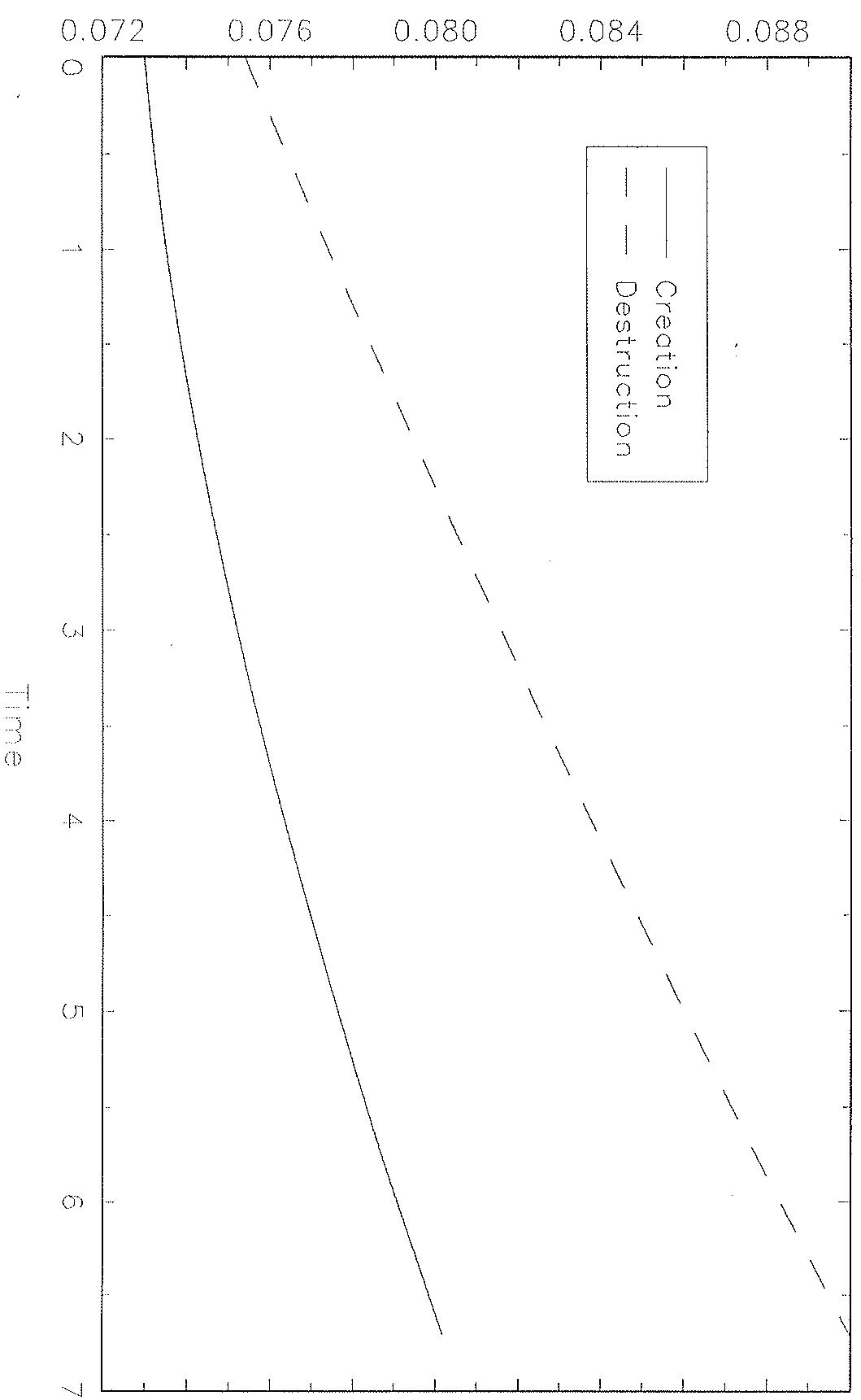
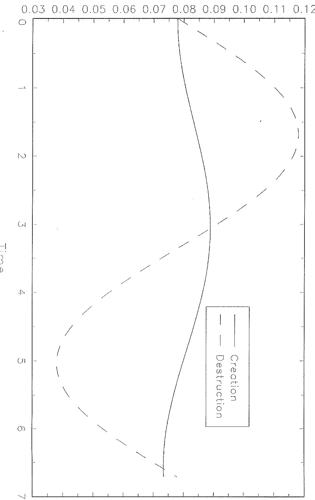
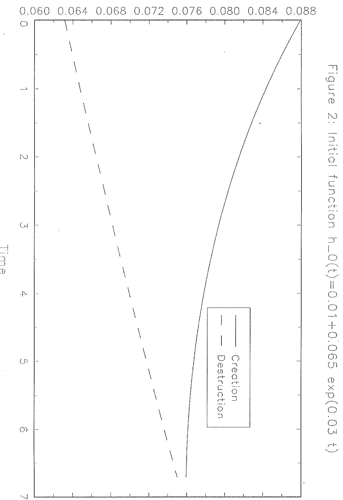
i) Depending on the parameters values , job creation and job destruction can be fully synchronized, fully decoupled or partially synchronized (or decoupled). For example, for , and , both job creation and job destruction increase over the interval . See this full synchronization case in Figure 1. For , and , we get a full decoupling case (see Figure 2): Job creation decreases whereas job destruction increases over the interval .

ii) The integral operator relating job creation to job destruction smoothes the dynamics of job creation with respect to those of job destruction. The smoothing effect is clear for example when , and , see Figure 3.

Both properties are far from surprising given the mathematical structure of our problem. From the economic point of view, these properties come from the fact that in our model the instantaneous variation of job creation is proportional to net job creation (the difference ), the proportionality factor being negative (equal to -a by (13)). The obtained proportionality is a direct consequence of the constancy of the optimal scrapping rule. If the optimal scrapping rule is constant, a high job creation in the past implies a high job destruction today. If past job creation is sufficiently high, current job creation will be small by equations (12) and current net job creation will be negative, which stimulates job creation by the proportionality rule mentioned just above. Accordingly, it is relatively easy to interpret the numerical cases illustrating Property i). Job creation is increasing in the past (over the interval ), which implies that job destruction will be increasing over the interval . If past job creation is sufficiently high (the case ), job creation will be relatively small over the interval and the resulting net job creation will be negative over the same interval. By the proportionality rule, job creation will increase over this interval as job destruction. We get the opposite results when past job creation is relatively small (the case ).

By fully synchronized (Resp. decoupled), we mean that the correlation between job creation and job destruction is always positive (Resp. negative) over the interval . By partially synchronized (or decoupled), we mean that the sign of the correlation between the two variables changes within the interval.

¿From the exposition above, it is clear that our properties i) and ii) result from the constancy of the optimal scrapping rule (or of the optimal lifetime of capital goods). In more general frameworks (with non-constant marginal hiring costs, with strictly concave utility functions or under non-stationary environments), the optimal scrapping rules are generally non-constant. This additional dynamic source will interact with the mechanisms underlying properties i) and ii), and the resulting dynamics compared to those of this paper will depend on the relative strength of the effects of the time dependent scrapping rules. For example, if the magnitude of the response of the optimal scrapping rules to changes in the exogenous environment is sufficiently small, our properties i) and ii) are unlikely to be altered a lot.

5 Conclusion

This paper is a theoretical contribution to the topic of job creation and job destruction. The ongoing research programs on the same topic have already pointed at a number of empirical and theoretical issues. This paper presents a basic framework for the discussion of these issues. To this end, we use a simplified version of Caballero and Hammour's model (1996). Especially, we assume that the marginal hiring cost is constant and we remove all exogenous fluctuations sources, which in turn allows us to focus exclusively on the implications of the endogenous fluctuations due to replacement investment. In contrast to the existing literature, our results are analytical. We show that the optimal scrapping rule (or the optimal lifetime of capital goods) is constant in such a framework and that job creation dynamics are driven by a simple backward-looking differential-difference equation. We prove that the latter equation gives rise to non-monotonic solution paths following the “echo principle”. The exact patterns of the solution paths depend on the initial job profiles of the considered economies.

Two main conclusions can be drawn from the performed analysis of the solution paths. First, job creation is smoother than job destruction in our basic framework, which is consistent with the empirical literature in the field. When business fluctuations are purely endogenous as in our framework, the increasing marginal hiring cost assumption is unnecessary to smooth out job creation. Secondly, depending on the initial job profile, job creation and job destruction can be either synchronized or decoupled at the inefficient decentralized equilibrium of our model. Therefore, the inefficiency of the decentralized equilibria does not imply necessarily that job creation and job destruction are decoupled. Our findings result fundamentally from the constancy of the optimal scrapping rule in our model. In more general frameworks (for example with non-stationary environments as in Caballero and Hammour (1996)), the optimal scrapping rules are generally non-constant. However, if the magnitude of the response of the optimal scrapping rules to changes in the exogenous environment is sufficiently small, our findings are unlikely to be altered a lot.

References

1. AGHION, Ph. and P. HOWITT (1992), “A Model of Growth through Creative Destruction”, Econometrica 60, 323-352.
2. AGHION, Ph. and P. HOWITT (1994), “Growth and Unemployment”, Review of Economic Studies 61, 477-494.
3. BELLMAN, R. and L. COOKE (1963), Differential-Difference Equations. Academic Press: New York.
4. BENHABIB, J. and A. RUSTICHINI (1991), “Vintage Capital, Investment, and Growth”, Journal of Economic Theory 55, 323-339.
5. BENHABIB, J. and A. RUSTICHINI (1993), “Vintage Capital Model of Investment and Growth: Theory and Evidence”, In Becker R. et al (eds.), General Equilibrium, Growth and Trade. II The Legacy of Lionel W. Mckenzie. Academic Press: New York.
6. BOERI, T. and J. CRAMER (1992), “Employment Growth, Incumbents and Entrants”, International Journal of Industrial Organization 10, 545-565.
7. BOUCEKKINE, R., M. GERMAIN and O. LICANDRO (1997-a), “Replacement Echoes in the Vintage Capital Growth Model”, Journal of Economic Theory 74, 333-348.
8. BOUCEKKINE, R., O. LICANDRO and C. PAUL (1997-b), “Differential-Difference Equations in Economics: On the Numerical Solution of Vintage Capital Growth Models”, Journal of Economic Dynamics and Control 21, 347-362.
9. CABALLERO, R. and M. HAMMOUR (1994), “The Cleansing Effect of Recessions”, American Economic Review 84, 1350-1368.
10. CABALLERO, R. and M. HAMMOUR (1996), “On the Timing and Efficiency of Creative Destruction”, Quarterly Journal of Economics 111, 805-851.
11. COOLEY, T., J. GREENWOOD and M. YOROKOGLU (1994), “The Replacement Problem”, Discussion Paper 95, Institute for Empirical Economics.
12. DAVIS, S. and J. HALTIWANGER (1990), “Gross Job Creation and Destruction: Microeconomic Evidence and Macroeconomic Implications”, NBER Macroeconomics Annual 5, 123-168.
13. DAVIS, S. and J. HALTIWANGER (1992), “Gross Job Creation, Gross Job Destruction, and Employment Reallocation”, Quarterly Journal of Economics 107, 819-864.
14. DOLADO, J-J. and R. GOMEZ (1995), “Creación y Destrucción de Empleo en el Sector Privado Manufacturado Español: Un Análisis Descriptivo”, Investigaciones Económicas 19, 371-393.
15. DOMS, M., T. DUNNE and M. ROBERTS (1995), “The role of Technology Use in the Survival and Growth of Manufacturing Plants”, International Journal of Industrial Organization 13, 523-542.
16. HULTEN, Ch. (1992), “Growth Accounting when Technical Change is Embodied in Capital”, American Economic Review 82, 964-980.
17. KONINGS, J. (1995), “Gross Job Creation and Gross Job Destruction in the UK Manufacturing Sector”, Oxford Bulletin of Economics and Statistics, forthcoming.
18. SOLOW, R., J. TOBIN, C. VON WEIZSACKER and M. YAARI (1966), “Neoclassical Growth with Fixed Factor Proportions”, Review of Economic Studies 33, 79-115.
19. VAN HILTEN, O. (1991), “The Optimal Lifetime of Capital Equipment”, Journal of Economic Theory 55, 449-454.

Appendix

Proof of Proposition 2: Since and , we have :

\[F (0) \leq T ^ {\intercal} (t) \leq \bar {F}\]

with

Applying the latter inequalities at , using (11) we get :

\[F (0) \leq J (t) \leq \bar {F}.\]

Given that function is increasing under Assumption 1, this yields :

\[F (F (0)) \leq T (t) \leq F (\bar {F}).\]

As before, we can apply the latter inequalities at , find new lower and upper bound for and establish new lower and upper bound for , . Repeating this reasoning, we can construct a sequence of lower bounds and upper bounds for , , such that,

\[\begin{array}{l l l} \forall n \geq 0 \text {and} t \geq 0 & X _ {n} \leq T (t) \leq Y _ {n}; \\ X _ {0} = F (0), & \text {and} X _ {n} = F (X _ {n - 1}) & \forall n \geq 1; \\ Y _ {0} = \bar {F}, & \text {and} Y _ {n} = F (Y _ {n - 1}) & \forall n \geq 1. \end{array}\]

Trivially, and . being strictly increasing, the sequence is decreasing and is increasing. Finally, observe that and , ; the two sequences are bounded. Since they are monotonic, both of them converge and, by construction of these sequences, the limits are equal to the unique fixed-point of function .

Proposition 5 (No jump property) Denoting , the solution path produced by the method of steps described above hold:

\[\forall k \in \aleph^ {*} \quad \lim _ {t \longrightarrow k T ^ {\circ}} h (t) = h (k T ^ {\circ})\tag{14}\]

Proof: Given the way the solution is computed by the method of steps, it is sufficient to prove the "No jump property" stated above to ensure the continuity of the solution paths at any strictly positive date. By construction of the method of steps, we have:

\[\lim _ {t \longrightarrow k T \circ} h (t) = \lim _ {t \longrightarrow k T \circ} h _ {k} (t).\]

For any , is the solution on of the ODE:

\[h ^ {\prime} (t) = - a \left(h (t) - h _ {k - 1} (t - T ^ {\circ})\right),\]

with given (either the initial function for or a previously computed solution for ) and

\[h ((k - 1) T ^ {\circ}) = a \left(1 - \int_ {(k - 2) T ^ {\circ}} ^ {(k - 1) T ^ {\circ}} h _ {k - 1} (\tau) d \tau\right).\]

Solving the ODE, we get:

\[h (t) = h _ {k} (t) = e ^ {- a t} \left[ e ^ {a (k - 1) T ^ {\circ}} h ((k - 1) T ^ {\circ}) + a \int_ {(k - 1) T ^ {\circ}} ^ {t} h _ {k - 1} (\tau - T ^ {\circ}) e ^ {a \tau} d \tau \right]\tag{15}\]

on . So:

\[\lim _ {t \longrightarrow k T ^ {\circ}} h _ {k} (t) = e ^ {- a k T ^ {\circ}} \left[ e ^ {a (k - 1) T ^ {\circ}} h ((k - 1) T ^ {\circ}) + a \int_ {(k - 1) T ^ {\circ}} ^ {k T ^ {\circ}} h _ {k - 1} (\tau - T ^ {\circ}) e ^ {a \tau} d \tau \right]\tag{16}\]

whereas

\[h \left(k T ^ {\circ}\right) = a \left(1 - \int_ {k T ^ {\circ} - T ^ {\circ}} ^ {k T ^ {\circ}} h (\tau) d \tau\right),\]

so that

\[h \left(k T ^ {\circ}\right) = a \left(1 - \int_ {(k - 1) T ^ {\circ}} ^ {k T ^ {\circ}} h _ {k} (\tau) d \tau\right).\]

Consider now the integral . Using (15), we can see that:

\[\begin{array}{r c l} I (k) & = & \frac {- h ((k - 1) T ^ {\circ})}{a} (e ^ {- a k T ^ {\circ}} - e ^ {- a (k - 1) T ^ {\circ}}) e ^ {- a (k - 1) T ^ {\circ}} + \\ & & + a \int_ {(k - 1) T ^ {\circ}} ^ {k T ^ {\circ}} e ^ {- a \tau} (\int_ {(k - 1) T ^ {\circ}} ^ {\tau} h _ {k - 1} (\upsilon - T ^ {\circ}) e ^ {a \upsilon} d \upsilon) d \tau , \end{array}\]

and by integrations by parts:

\[\begin{array}{r c l} I (k) & = & \frac {- h ((k - 1) T ^ {\circ})}{a} \left(e ^ {- a k T ^ {\circ}} - e ^ {- a (k - 1) T ^ {\circ}}\right) e ^ {- a (k - 1) T ^ {\circ}} + \\ & & + a \left(\frac {- e ^ {- a k T ^ {\circ}}}{a} \int_ {(k - 1) T ^ {\circ}} ^ {k T ^ {\circ}} h _ {k - 1} (\tau - T ^ {\circ}) e ^ {a \tau} d \tau + \frac {1}{a} \int_ {(k - 1) T ^ {\circ}} ^ {k T ^ {\circ}} h _ {k - 1} (\tau - T ^ {\circ}) d \tau\right). \end{array}\]

Using the fact that

\[h \left((k - 1) T ^ {\circ}\right) = a \left(1 - \int_ {(k - 2) T ^ {\circ}} ^ {(k - 1) T ^ {\circ}} h _ {k - 1} (\tau) d \tau\right) = a \left(1 - \int_ {(k - 1) T ^ {\circ}} ^ {k T ^ {\circ}} h _ {k - 1} (\tau - T ^ {\circ}) d \tau\right),\]

we get:

\[I (k) = 1 - \left[ \frac {- h ((k - 1) T ^ {\circ}) e ^ {a (k - 1) T ^ {\circ}}}{a} + \int_ {(k - 1) T ^ {\circ}} ^ {k T ^ {\circ}} h _ {k - 1} (\tau - T ^ {\circ}) e ^ {a \tau} d \tau \right].\]

So:

\[h \left(k T ^ {\circ}\right) = a (1 - I (k)) = \lim _ {t \rightarrow k T ^ {\circ}} h _ {k} (t)\]

by comparison with (16).

COLECCION RESUMENES

96-02: “Evidencia empírica de sustituibilidad entre los componentes sectoriales del ahorro nacional en algunos países de la Unión Europea”, Isabel Argimón.

96-01: “El mercado de depósitos español (1985-1994): Bancos versus Cajas de Ahorro”, Juan Coello.

TEXTOS EXPRESS

97-02: "II Encuesta sobre la UEM InterMoney-FEDEA: Resultados", C. Arenillas, J. A. Herce, J. A. Ketterer, S. Sosvilla y D. Vegara.

97-01: “La cuestión de las pensiones”, José A. Herce.

DOCUMENTOS DE TRABAJO

97-13: “Replacement investment, endogenous fluctuations and the dynamics of job creation and job destruction”, Raouf Boucekkine, Fernando del Rio y Omar Licandro.

97-12: “La demanda de automóviles en España: Un análisis de la evolución y variabilidad de las tasas de reemplazo”, Omar Licandro, Antonio R. Sampayo.

97-11: “Respuesta de los tipos de interés nominales españoles a shocks de inflación esperada y de tipos de interés real ex-ante: Una aplicación VAR estructural”, Vicente Esteve.

97-10: “Convergence in fiscal pressure across EU countries”, Vicente Esteve, Simón Sosvilla y Cecilio Tamarit.

97-09: “Evaluación de los efectos macroeconómicos del fondo de cohesión en España”, Juan Carlos Císcar.

97-08: “Creative destruction, investment volatility, and the average age of capital”, R. Boucekkine, M. Germain, O. Licandro y A. Magnus.

97-07: “Spatially and intertemporally efficient waste management: The costs of interstate flow control”, Eduardo Ley, Molly K. Macauley y Stephen W. Salant.

97-06: “Are there any special features in the Spanish business cycle?, Luis Puch y Omar Licandro.

97-05: “Los factores específicos del paro en Andalucía” Juan F. Jimeno.

97-04: “The effects of minimum bargained wages on earnings: Evidence from Spain”, Juan J. Dolado, Florentino Felgueroso y Juan F. Jimeno.

97-03: “Convergence in social protection benefits across EU countries”, Javier Alonso, Miguel Angel Galindo y Simón Sosvilla.

97-02: “Public-good productivity differentials and non-cooperative public-good provision”, Eduardo Ley.

97-01: “Paridad del poder adquisitivo: Una reconsideración”, F. J. Ledesma, M. Navarro, J. V. Pérez y S. Sosvilla.

96-28: “Urbanization and growth”, Juan J. de Lucio.

96-27: “Efectos macroeconómicos del mercado único europeo: Un análisis basado en el modelo HERMIN”, Simón Sosvilla-Rivero y José. Herce.

96-26: “Capacity and access pricing strategies: An argument for the liberalization of telecommunication infrastructure”, A. Urbano, G. Olcina y Y. Tauman.

96-25: “La reforma de las pensiones en España: Aspectos analíticos y aplicados”, José A. Herce.

96-24: “Transitional effects of a pension system change in Spain”, José M. Bailén y Joan Gil.

96-23: “Convergencia real en la Unión Europea: Un análisis de series temporales”, Vicente Esteve y Vicente J. Pallardó.

96-22: “Monetary Union and european unemployment”, José Viñals y Juan F. Jimeno.

96-21: “El equilibrio financiero de un sistema de reparto de pensiones de jubilación: Una aplicación al caso español”, Juan F. Jimeno y Omar Licandro.